p. bhogale
 These notes are meant to impliment little examples from Francois Fleuret's Little Book of Deep Learning (pdf link) in r-torch. I'm writing these as a fun way to dive into torch in R while surveying DL quickly.
You'll need to have the book with you to understand these notes, but since it is available freely, that ought not to be an issue.
Basis function regression
We will generate synthetic data that is similar to the example shown in the book:
# Number of samples
n <- 50

# Randomly distributed x values from -1 to 1
set.seed(123) # for reproducibility
x <- runif(n, min = -1, max = 1)
##
## Attaching package: 'stats'
## The following objects are masked from 'package:dplyr':
##
##     filter, lag
x <- sort(x) # Sorting for plotting purposes
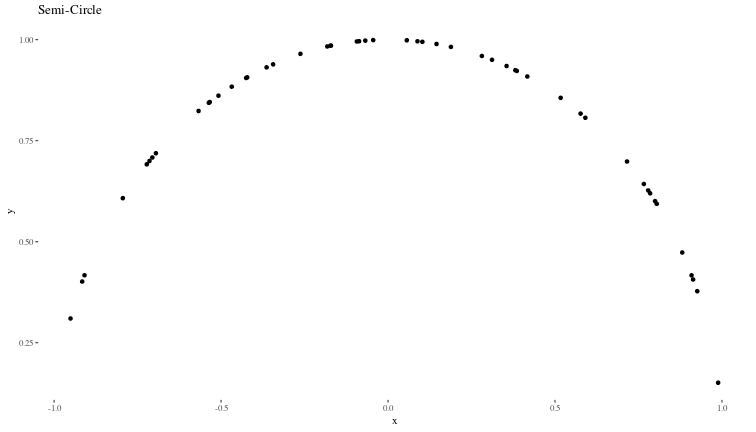
# y values as the semi-circle
y <- sqrt(1 - x^2)
# Plotting the original semi-circle with randomly distributed x
data <- data.frame(x = x, y = y)
ggplot(data, aes(x, y)) +
geom_point() +
ggtitle("Semi-Circle") +
theme_tufte()
Following the book, we use gaussian kernels as the basis functions to fit \(y \sim f(x;w)\), where \(w\) are the weights of the basis functions.
# Define Gaussian basis functions
basis_functions <- function(x, centers, scale = 0.1) {
  exp(-((x - centers)^2) / (2 * scale^2))
}

# Centers of the Gaussian kernels, these do cover the region of space we are interested in
centers <- seq(-1, 1, length.out = 10)
Now, we define our model for \(y\), which, for basis function regression, is a linear combination of the basis functions initialized with random weights \(w\).
# Initial random weights
weightss <- torch_randn(length(centers), requires_grad = TRUE)

# Calculate the model output
model_y <- function(x) {
  # Convert x to a torch tensor if it isn't already one
  x_tensor <- torch_tensor(x)

  # Create a tensor for the basis functions evaluated at each x
  # Resulting tensor will have size [length(x), length(centers)]
  basis_matrix <- torch_stack(lapply(centers, function(c) basis_functions(x_tensor, c)), dim = 2)

  # Calculate the output using matrix multiplication
  # basis_matrix is [n, 10] and weights is [10, 1]
  y_pred <- torch_matmul(basis_matrix, weightss)

  # Flatten the output to match the dimension of y
  return(y_pred)
}
Now,we will use gradient descent to minimise the MSE between the model and the real values of \(y\) to obtain the optimal weights \(w^*\).
# Learning rate
lr <- 0.01

# Gradient descent loop
for (epoch in 1:5000) {
  y_pred <- model_y(x)

  op <- nnf_mse_loss(y_pred, torch_tensor(y))

  # Backpropagation
  op$backward()

  # Update weights
  with_no_grad({
    weightss$sub_(lr * weightss$grad)
    weightss$grad$zero_()
  })
}
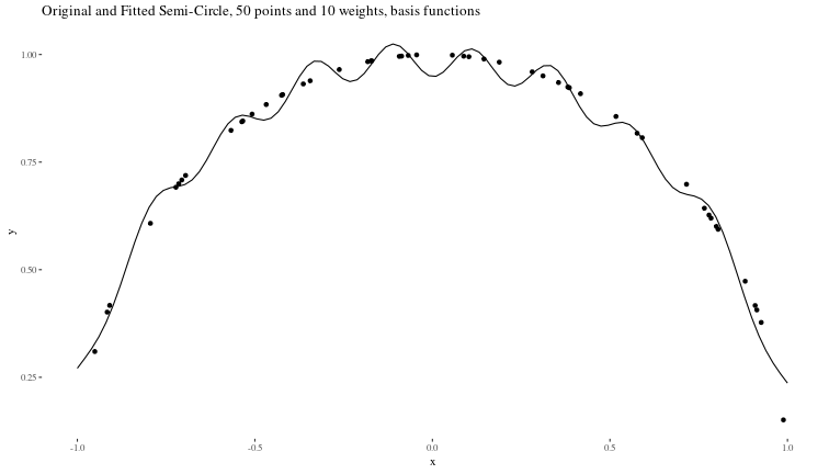
Now, we can see how good our predictions are:
# Get model predictions
fin_x <- seq(-1,1,length.out=100)
final_y <- model_y(fin_x)

# Plotting
predicted_data <- data.frame(x = fin_x, y = as.numeric(final_y))
ggplot() +
  geom_point(data = data, aes(x, y)) +
  geom_line(data = predicted_data, aes(x, y)) +
  ggtitle("Original and Fitted Semi-Circle, 50 points and 10 weights, basis functions") +
  theme_tufte()
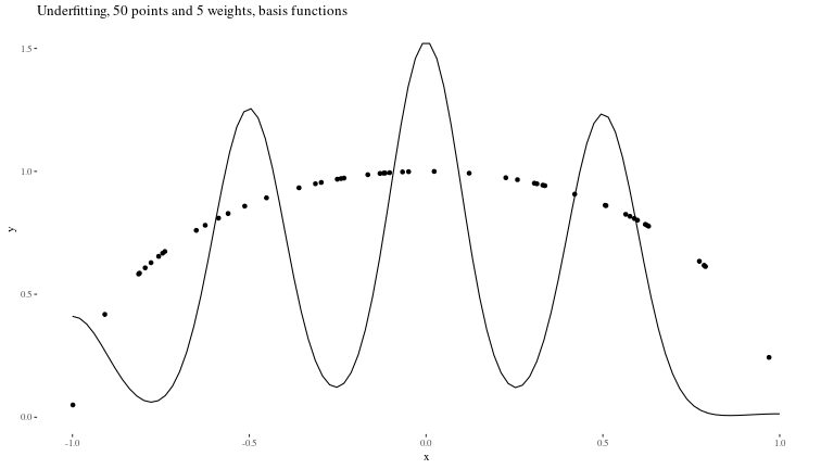
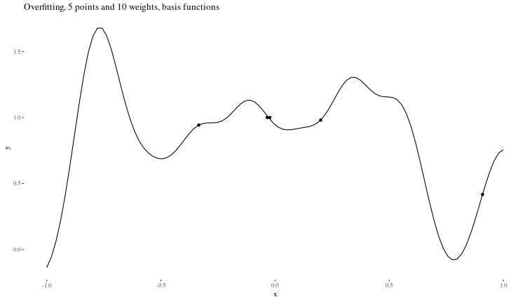
Underfitting When the model is too small to capture the features of the data (in our case, too few weights)
Overfitting When there is too little data to properly constrain the parameters of a larger model.
Autoregressive models
Let us generate data that looks similar to that shown in section 3.5 of the book.
# Function to generate C-shaped data
generate_c_data <- function(n, x_offset, y_offset, y_scale, label, xflipaxis) {
  theta <- runif(n, pi/2, 3*pi/2)  # Angle for C shape
  x <- cos(theta) + rnorm(n, mean = 0, sd = 0.1) + x_offset
  if(xflipaxis==T){
    x <- 1-x
  }
  y <- sin(theta) * y_scale + rnorm(n, mean = 0, sd = 0.1) + y_offset
  data.frame(x = x, y = y, label = label)
}

# Number of points per class
n_points <- 1000

# Generate data for both classes
data_class_1 <- generate_c_data(n_points, x_offset = 0,
                                y_offset = 0, y_scale = 1, label = 1,
                                xflipaxis = F)
data_class_0 <- generate_c_data(n_points, x_offset = 1.25,
                                y_offset = -1.0, y_scale = -1, label = 2,
                                xflipaxis = T)  # Mirrored and adjusted

# Combine data
data <- rbind(data_class_0, data_class_1)

# Plotting the data
ggplot(data, aes(x, y, color = as.factor(label))) +
  geom_point(alpha = 0.7, size = 3) +
  labs(title = "Adjusted C-shaped Data for Classification", x = "X axis", y = "Y axis") +
  theme_tufte()
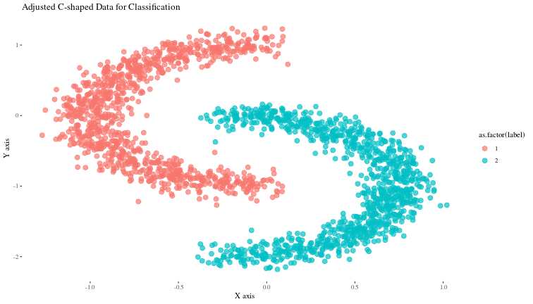
Now, we can build a very simple neural net to classify these points and try to visualize what the trained net is doing at each layer.
Now, let us see (visually) how well the model predicts some new synthetic data generated similarly.
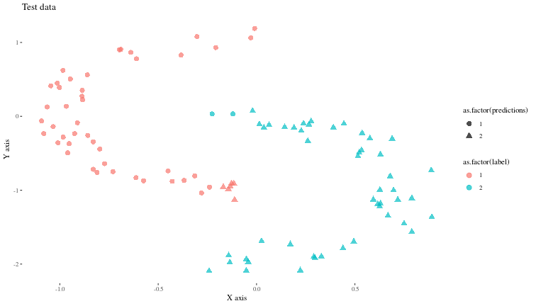
TODO: I have not yet figured out a way to access model activations when the model is trained with luz.
Architectures
Multi Layer Perceptrons
This is a neural net that has a series of fully connected layers seperated by activations. We will illustrate an MLP using the Penguins dataset, where we try to predict the species of a penguin from some features. Example adapted from the excellent Deep Learning with R Torch book.
library(palmerpenguins)

penguins <- na.omit(penguins)
ds <- tensor_dataset(
  torch_tensor(as.matrix(penguins[, 3:6])),
  torch_tensor(
    as.integer(penguins$species)
  )$to(torch_long())
)

n_class <- penguins$species |> unique() |> length() |> as.numeric()
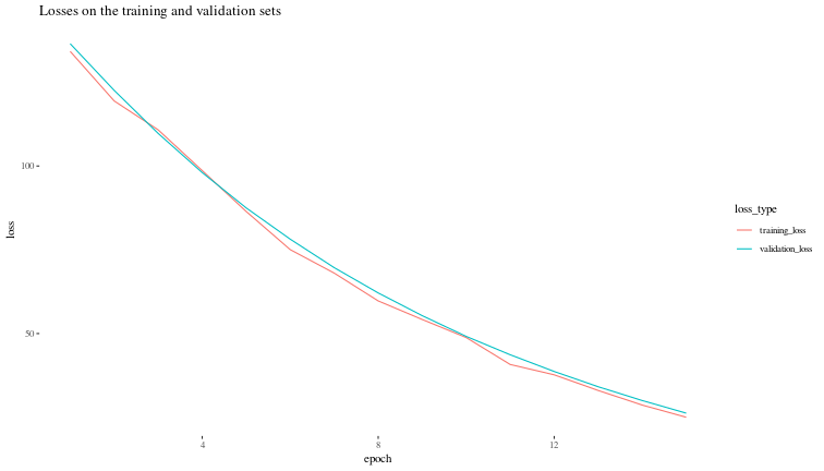
Now, we train a simple MLP on 75% of this dataset.
mlpnet <- nn_module(
  "MLPnet",
  initialize = function(din, dhidden1, dhidden2, dhidden3, n_class) {
    self$net <- nn_sequential(
      nn_linear(din, dhidden1),
      nn_relu(),
      nn_linear(dhidden1, dhidden2),
      nn_relu(),
      nn_linear(dhidden2, dhidden3),
      nn_relu(),
      nn_linear(dhidden3, n_class)
    )
  },
  forward = function(x) {
    self$net(x)
  }
)
Now, let us visualize the validation loss during the training process.