A first foray into probabilistic programming with Greta

Models and modelling

Much of science - physical and social - is devoted to positing mechanisms that explain how the data we observe are generated. In a classic example, after Tycho Brahe made detailed observations of planetary motion (here is data on mars), Johannes Kepler posited laws of planetary motion that explained how this data were generated. Effectively, modelling is the art of constructing data generators that help us understand and predict.

Statistical models are one class of models that aim to construct - given some observed data - the probability distribution from which the data were drawn. That is, given a sample of data, a statistical model is a hypothesis about how this data were generated. In practice, this happens in two steps :
- constructing a hypothesis, or a model \(H\) parametrized by some parameters \(\theta\),
- finding (inferring) the distribution of parameters \(\theta\) or, the most suitable parameters \(\theta\) given the observed data

What parameters are "most suitable" is indicated (in a particular sense of the word "suitable" will become clear in the following discussion) by the likelihood function that quantifies how probable the observed data set is, for a given hypothesis parametrized by some particular parameters \(H_{\theta}\). Understandably, we want to find parameters such that the observed data is the most likely, this is called maximum likelihood estimation.

Since all but the simplest models are analytically intractable (i.e., the maximum of the likelihood function needs to be evaluated numerically and parameter distributions are even harder to compute) it makes sense to construct general rules and syntax to easily define statistical models and quickly infer their parameters. This is the field of probabilistic programming.

Probabilistic programming

The probabilistic programming language (PPL) has two tasks :

1. be able to construct a useful class of statistical models
2. be able to infer the parameters (and their distributions) of this class of models given some observed data.

As has been explained in this excellent paper introducing the PPL Edward that is based on Python and Tensorflow, some PPLs restrict the class of models they allow in order to optimize the inference algorithm, while other emphasize expressiveness and sacrifice performance of the inference algorithms. Modern PPLs like Edward, Pyro, and the R based Greta use the robust infrastructure (hardware and software) that was first developed in the context of deep learning and thus ensure scalability and performance while being expressive.

The tensor and the computational graph

The fundamental data structure of this group of languages is the tensor which is just a multidimensional array. Data, model parameters, samples from distributions are all stored in tensors. All the manipulations that go into the construction of the output tensor constitute the computational graph (see this for an exceptionally clear exposition of the concept) associated with that tensor.

Data and parameter tensors are inputs to the computational graph. In the context of deep learning, "training" consists of the following steps :

1. Randomly initializing the parameter tensors
2. Computing the output
3. Measuring the error compared to the real/desired output
4. Tweaking the parameter tensors to reduce the error.

The algorithm that does this is called back propagation. Thus, the objective in deep learning or machine learning is to obtain the best values (in the sense of that they minimize error on the training set) of the parameters given some data.

The objective of probabilistic modelling is subtly different. The aim here is to obtain the distribution (called posterior distribution) of parameters, given the data. If we denote the data by \(D\), Bayes theorem relates (for a particular hypothesis about how the data were generated \(H\)), the likelihood of the data given some parameters \(P(D|\theta,H)\), our prior expectations about how the parameters are distributed \(P(\theta)\) and the posterior distribution of the parameters themselves \(P(\theta|D,H)\) :

The priors \(P(\theta)\) do not depend on the data and encode "domain knowledge" while the probability of the data set \(P(D)\) over the whole parameter space is (typically) a high dimensional integral given by

Intuitively, we can see that the most likely parameters given the data, i.e. the parameters \(\theta\) which maximize \(P(\theta|D,H)\) ought to correspond to the sense of "best" or "most suitable" described above. From Bayes theorem, it is clear that the posterior distribution is directly proportional to the likelihood \(P(\theta|D,H) \propto P(D|\theta,H)\). Thus, maximizing likelihood is one way to get estimates of the "most likely parameters" (in the limit of infinite data), but computing the full distribution \(P(\theta|D,H)\) involves dealing with the difficult integral for \(P(D|H)\).

Bayesian prediction and MCMC

Prediction in this framework is also fundamentally different from typical machine learning model. The probability of a new data point \(d\),

which consists of the expectation value of the new data point over the whole distribution of parameters given the observed data (the posterior distribution calculated obtained from the solution to the inference problem), instead of a value calculated by plugging in the "learned parameter values" into the machine learning model.

The integrals needed for inference (\(P(D|H) = \int P(D,\theta|H)d\theta\) as well as prediction \(P(d|D,H) = \int P(d|\theta,H)P(\theta|D,H)d\theta\) need to be evaluated over the entire parameter space of the model which can be very high dimensional. Markov Chain Monte Carlo methods are used to approximate these integrals. This is an excellent overview of modern Hamiltonian Monte Carlo methods while this provides wonderful perspective from the dawn of the field. Both papers are long but eminently readable and highly recommended.

Clearly then, along with the computational graph to define models, a PPL needs a good MCMC algorithm (or another inference algorithm) to compute the high dimensional integrals needed to infer as well as perform a prediction on a general probabilistic model.

A broad overview of Bayesian machine learning is available here (PDF) and here

Now, we illustrate some of these points using the simplest possible example, linear regression.

Basic linear regression.

We will generate artificial data with known parameters, so that we can check if Greta (the PPL we are using for this article) gets it right later.

Generating fake data to fit a model to

length_of_data <- 100
sd_eps <- pi^exp(1)
intercept <- -5.0
slope <- pi
x <- seq(-10*pi, 10*pi, length.out = length_of_data)
y <- intercept + slope*x + rnorm(n = length_of_data, mean = 0, sd = sd_eps)
data <- data_frame(y = y, x = x)
ggplot(data, aes(x = x, y = y, colour = "simulated dependent variable")) +
  geom_point() +
  geom_smooth(method = 'lm') +
  ggtitle("Fake experimental data") +
  ggthemes::theme_economist()

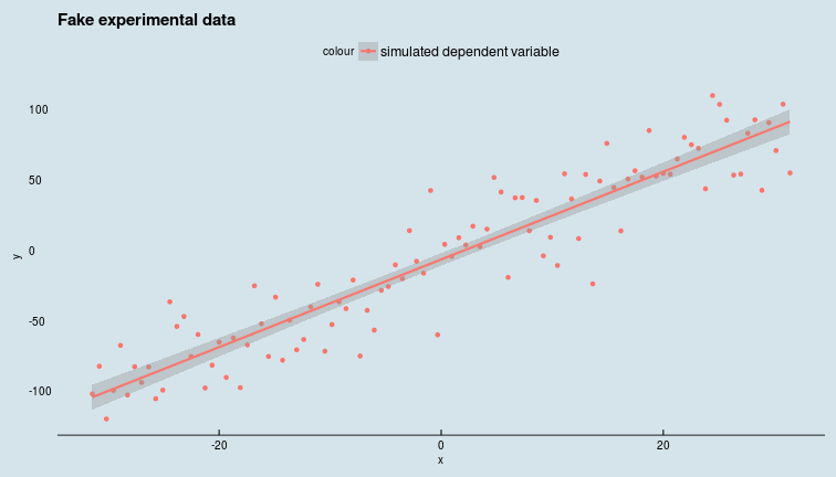
Given this data, we want to write Greta code to infer the posterior distributions of the model parameters.

Defining clueless priors for model parameters

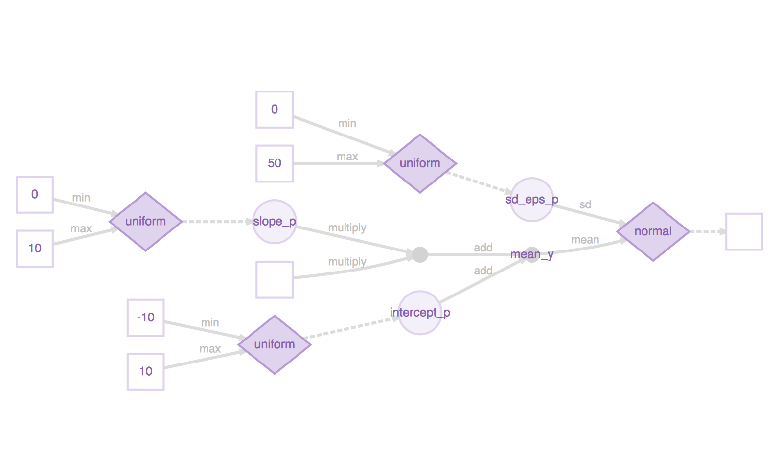
In this case, the parameters of our model are simple, but in principle, they can be arbitrary tensors. Since we really don't know anything about the prior distributions of our parameters, we look at the experimental data and take rough, uniform priors.

intercept_p <- uniform(-10, 10)
sd_eps_p <- uniform(0, 50)
slope_p <- uniform(0, 10)

Defining the model

mean_y <- intercept_p+slope_p*x
distribution(y) <- normal(mean_y, sd_eps_p)

Here, we hypothesize that the target variable \(y\) is linearly dependent on some independent variable \(x\) with a noise term drawn from a Gaussian distribution whose standard deviation is also a parameter of the model.

Under the hood, Greta has constructed a computational graph that encapsulates all these operations, and defines the process of computing the target \(y\) starting from the prior distributions of our input variables. We plot this computational graph below :

our_model <- model(intercept_p, slope_p, sd_eps_p)
our_model %>% plot()

Inference

There are two distinct types of inference possible,

1. Sampling from the full posterior distribution for the parameters given the data and the model.
2. Maximizing likelihood to compute "most probable" parameters given the data and the model.

Sampling from the posterior distribution of parameters with MCMC

num_samples <- 1000
param_draws <- mcmc(our_model, n_samples = num_samples, warmup = num_samples / 10)

and plot the densities of samples drawn from the parameter posterior distributions, and the parameter fits.

mcmc_dens(param_draws)

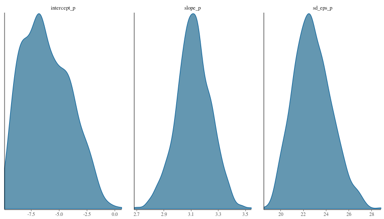
mcmc_intervals(param_draws)

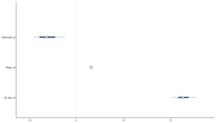
By inspection, it looks like the HMC has found reasonable values for our model parameters and their posterior distributions.

Most probable parameters

Explicitly, the mean estimates can be computed from the param_draws data structure, or via the greta::opt function.

param_draws_df <- as_data_frame(param_draws[[1]])
param_estimates <- param_draws_df %>% 
  summarise_all(mean)
param_estimates %>% print()

## # A tibble: 1 x 3
##   intercept_p slope_p sd_eps_p
##         <dbl>   <dbl>    <dbl>
## 1       -6.12    3.12     22.8

opt_params <- opt(our_model)
opt_params$par %>% print()

## intercept_p     slope_p    sd_eps_p 
##   -6.686146    3.187089   23.300232

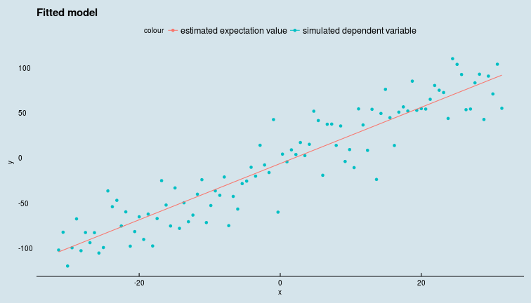
Bayesian prediction

Bayesian prediction is implemented via the calculate() function available in the latest release of greta on github. This generates a prediction on \(y\) for each draw from the posterior distribution of the parameters (see previous section). Taking the expectation over this distribution of predictions gives us the mean value of the target variable \(y\) but we have the whole distribution of \(y\) available to us if we need to analyse it.

mean_y_plot <- intercept_p+slope_p*x
mean_y_plot_draws <- calculate(mean_y_plot, param_draws)
mean_y_est <- colMeans(mean_y_plot_draws[[1]])
data_pred <- data %>% mutate(y_fit = mean_y_est)
ggplot(data_pred) +
  geom_point(aes(x,y,colour = "simulated dependent variable")) +
  geom_line(aes(x,y_fit, colour = "estimated expectation value")) +
  ggtitle("Fitted model") +
  ggthemes::theme_economist()

Further exploration

1. The most mature PPL out there (with good R bindings) is Stan. There is a lot of material available, and it might be a good place to start to pick up some intuition. See this page.
2. This is a good intro to the role of MCMC in inference.
3. These video lectures on statistical rethinking emphasizing Bayesian statistics also seem interesting.