"Basics of conformal prediction in time series data"

Reading material

Please read the previous blogpost for basics of conformal inference and more reading material.
This post makes use of the conformalForecast package introduced in the paper published just 10 days ago by Wang and Hyndman.
For a more general overview of time series forecasting, please see this excellent book by Hyndman.
Frank Hull's R code for Valeriy Manokhin's book.

Conformal prediction is a powerful, non-parametric approach to constructing prediction intervals that provide reliable coverage without requiring strong assumptions about the data distribution (see the previous post for an introduction and reading material). For time series forecasting, where data is temporally correlated, conformal prediction methods must adapt to these correlations to achieve accurate and reliable intervals.

We will first generate time series data and illustrate a couple of classical forecasting techniques before moving to conformal methods.

Generating simple time series data

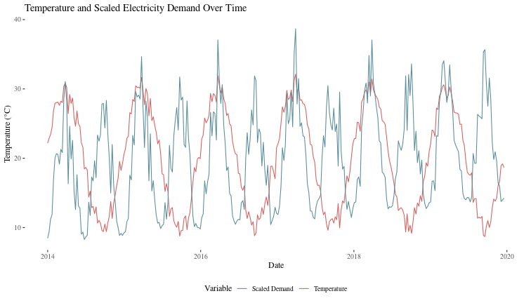
Let's create a synthetic dataset that mimics real-world electricity demand and temperature patterns, where demand is influenced by temperature in a U-shaped relationship (higher demand at both very low and very high temperatures):

set.seed(2024)
n <- 52*6  # 6 years of weekly data
time <- 1:n
holdout_prop <- 0.8
level_conf <- 0.8

# Generate synthetic temperature data with seasonal pattern
temperature <- 20 + 10 * sin(2 * pi * time / 52) + rnorm(n, sd = 1)

# Generate electricity demand influenced by temperature (U-shaped relationship)
temp_effect <- 2000 + 100 * (temperature - 20)^2
demand <- temp_effect + 500 * sin(2 * pi * time / 52) + 
  50 * time / 52 + rnorm(n, sd = 150) + (10*time)

# Organize data as time series and separate into training and test sets
data <- tibble(
  date = seq(as.Date("2014-01-01"), by = "week", length.out = n),
  temperature = temperature,
  demand = demand
)

Let's examine our data. First, let's look at the time series patterns:

ggplot(data, aes(x = date)) +
  geom_line(aes(y = temperature, color = "Temperature")) +
  geom_line(aes(y = scale(demand)[,1] * sd(temperature) + mean(temperature), 
                color = "Scaled Demand")) +
  scale_color_manual(values = c("Temperature" = "#D95F5F", "Scaled Demand" = "#5A8D9B")) +
  labs(title = "Temperature and Scaled Electricity Demand Over Time", x = "Date",
       y = "Temperature (°C)", color = "Variable") +
  theme_tufte(base_size = 12) +
  theme(legend.position = "bottom")

center

The `modeltime` workflow for time series forecasting

We will quickly show how to use the modeltime package for time series forecasts. We start by converting the data to a tsibble, an R object for time series dataframes.

data_ts <- data |> 
  mutate(date = as_date(date)) |> 
  as_tsibble(index = date) |> 
  rename(demand = demand, temperature = temperature)

data_split <- initial_time_split(data, prop = holdout_prop)
train_set <- training(data_split)
holdout <- testing(data_split)
cal_set <- initial_time_split(holdout, prop = holdout_prop) |> training()
test_set <- initial_time_split(holdout, prop = holdout_prop) |> testing()

In order to check how well we are doing ex-ante, we will need to forecast the temperature into the future, to understand demand.

temp_model_prophet <- prophet_reg() |> 
  set_engine(engine = "prophet", yearly.seasonality=TRUE) |> 
  fit(temperature ~ date, data = train_set)

temp_model_tbl <- modeltime_table(temp_model_prophet)

temp_forecast_tbl <- temp_model_tbl |> 
  modeltime_forecast(new_data = holdout, actual_data = data)

temp_forecast_tbl |> 
  plot_modeltime_forecast(.legend_show = FALSE, .title = "Temperature Forecast", .interactive = FALSE)

center

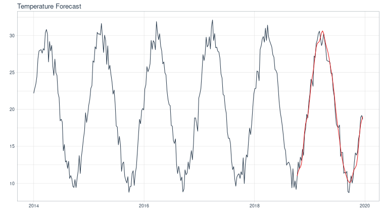
Now, we will need to replace the temperatures in the holdout, calibration and test sets with our temperature forecasts to ensure that our demand forecasts are ex-ante.

holdout$temperature <- {temp_forecast_tbl |> filter(.key == "prediction")}$.value
cal_set <- initial_time_split(holdout, prop = holdout_prop) |> training()
test_set <- initial_time_split(holdout, prop = holdout_prop) |> testing()
data_exante <- bind_rows(train_set, holdout)

Now, we create a prophet model with temperature as an exogenous variable and calibrate it on the calibration set data.

model_prophet <- prophet_reg() |> 
    set_engine(engine = "prophet", yearly.seasonality=TRUE) |> 
    fit(demand ~ date+temperature, data = train_set)

model_tbl <- modeltime_table(model_prophet)

calibration_tbl <- model_tbl |> 
  modeltime_calibrate(new_data = cal_set, quiet = FALSE)

Now, lets see what the forecast looks like with conformal intervals calculated by modeltime's built in conformal inference scheme.

forecast_tbl <- calibration_tbl |> 
  modeltime_forecast(new_data = test_set, 
                     actual_data = data_exante,
                     conf_method  = "conformal_default", 
                     conf_interval = level_conf, 
                     keep_data  = TRUE)
forecast_tbl |> 
  tail(nrow(test_set)*4) |> 
  plot_modeltime_forecast(.legend_show = TRUE, .title = "Demand Forecast", .interactive = FALSE)

center

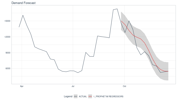
We see that the forecast remains equally confident far into the future which seems wrong (the regularity of the data notwithstanding), and the confidence intervals are symmetric around the mean

The modeltime workflow does calibrate the confidence intervals on samples outside the training set, so the coverage is not terrible.

In the following sections, we will address some of these aspects using conformal methods for multi timestep prediction using the conformalForecast package, and describe the AcMCP method, introduced in Wang and Hyndman’s paper.

Split Conformal Inference in Time Series

In traditional split conformal inference, we:

Split the data into a Training Set for model fitting and a Calibration Set to compute prediction intervals.
For each point in the calibration set, we calculate a nonconformity score (typically the absolute forecast error) to quantify the forecast's deviation from the observed values.
By taking a quantile of these scores, we construct prediction intervals around the forecasts.

What we did above with modeltime calibrating on the test set was exactly

However, time series data introduces unique challenges:

Forecast uncertainty increases with the forecast horizon due to accumulated prediction errors.
To adapt conformal prediction for time series, we use the sequential split approach, which respects the order of data points and maintains the temporal structure in the data.

Recipe for Split Conformal Prediction

Select Model and Forecast Horizon: Choose a forecasting model (e.g., ARIMA, Prophet) and decide on the forecast horizon $H$.
Split Data Sequentially: Divide the data sequentially into a training Set: for fitting the model and a calibration Set to calculate nonconformity scores.
Fit Model on Training Set: Train the model on the training set, then use it to generate predictions for points in the calibration set.
Calculate Nonconformity Scores: For each calibration point $y_{t+h}$, calculate the forecast $\hat{y}_{t+h|t}$ and the nonconformity score:
$$s_{t+h|t} = |y_{t+h} - \hat{y}_{t+h|t}|$$
Construct Prediction Intervals: First select a confidence level $1 - \alpha$. Then, find the $(1 - \alpha)$ th quantile of nonconformity scores to construct intervals for future points:
$$ \hat{C}_{t+h|t} = [\hat{y}_{t+h|t} - Q_{1-\alpha}, \hat{y}_{t+h|t} + Q_{1-\alpha}] $$

In time series forecasting, prediction intervals ideally widen for forecasts further into the future to capture the increased uncertainty over time. Standard split conformal prediction doesn’t account for this, as it uses a single quantile of nonconformity scores for all horizons. However, various methods address this limitation by widening intervals adaptively:

Horizon-Dependent Quantiles

Using horizon-specific nonconformity quantiles, we can tailor intervals to be wider for longer forecast horizons.

Recipe:

For each forecast horizon $h$, calculate separate quantiles $Q_{1-\alpha}^{(h)}$ based on the nonconformity scores for that specific horizon.
Define prediction intervals that adapt to each horizon:
$$ \hat{C}_{t+h|t} = [\hat{y}_{t+h|t} - Q_{1-\alpha}^{(h)}, \hat{y}_{t+h|t} + Q_{1-\alpha}^{(h)}] $$
This approach allows intervals to widen as the forecast horizon increases, reflecting higher uncertainty.

Online Conformal Inference for Multi-step Time Series Predictions

Creating prediction intervals that account for the uncertainty in predictions is challenging in time series because data points are correlated across time, violating the data exchangeability assumptions of traditional conformal methods. In particular, for multi-step forecasting (predicting $t+1, t+2, \ldots, t+H$), each interval needs to reflect both:

The growing uncertainty of further predictions.
The dependencies between errors at different steps ahead.

In online conformal inference for multi-step predictions, intervals are recursively updated as new observations arrive. This lets intervals adapt to shifts in data patterns, improving the long-term accuracy of coverage over time.

The AcMCP (Autocorrelated Multi-step Conformal Prediction) Method

The AcMCP method by Wang and Hyndman (2024) builds on these ideas by incorporating autocorrelations in multi-step forecast errors, unlike simpler methods that treat each forecast step independently. AcMCP produces statistically efficient prediction intervals by integrating these dependencies into the interval calculations, which is crucial for time series data.

Recipe

Modeling Forecast Error Structure:
- For an $h$-step-ahead prediction, AcMCP assumes that errors follow an MA($h-1$) structure, meaning the current error depends on the past $h-1$ steps.
- This structure is captured as:
  $$ e_{t+h|t} = \omega_{t+h} + \theta_1 \omega_{t+h-1} + \cdots + \theta_{h-1} \omega_{t+1}, $$
  where $\omega_t$ is random noise and $\theta$ terms reflect the error dependencies.
Updating Quantile Estimates: AcMCP updates the interval’s quantile estimate $q_{t+h|t}$ in real time, accounting for recent errors and their correlations. This update is key to keeping the interval valid over multiple steps and adapting to new information.
Combining Multiple Models
- An MA($h-1$) model trained on recent $h$-step-ahead errors to capture the correlation in errors.
- A linear regression model that uses recent errors to forecast future errors.

This combination enables AcMCP to capture both immediate and multi-step dependencies, refining prediction intervals as each new observation arrives.

Now, we illustrate the use of AcMCP using the conformalForecast package that accompanies the Wang and Hyndman (2024) paper.

horizon <- nrow(test_set)
# function that makes predictons of demand
demand_forecast <- function(y, h, level, xreg, newxreg) {
    model <- auto.arima(y, xreg = xreg)
    # Forecast using future temperature values
    fc <- forecast(model, h = h, xreg = newxreg, level = level)
    return(fc)  # Returns a forecast object
}

# Generateing rolling forecast and errors on the given data
demand_fc <- cvforecast(
    y = ts({rbind(train_set, cal_set) |> select(demand)}, frequency = 52),
    forecastfun = demand_forecast,
    h = horizon,
    level = c(level_conf),
    xreg = matrix({data_exante$temperature |> head(nrow(train_set)+nrow(cal_set)+horizon)}, ncol = 1),
    initial = 10, 
    window = horizon*10
)

We use the forecasting function created above to generate conformal predictions.

cal_window <- max(10, horizon*5)
symm <- FALSE
roll <- FALSE
Tg <- 4
delta <- 0.01
Csat <- 2 / pi * (ceiling(log(Tg) * delta) - 1 / log(Tg))
KI <- 0.5
lr <- 0.1

acmcp <- mcp(demand_fc, alpha = 1 - 0.01 * demand_fc$level,
             ncal = cal_window, rolling = roll,
             integrate = TRUE, scorecast = TRUE,
             lr = lr, KI = KI, Csat = Csat)

Lets see how this compares with the forecasts from the modeltime prophet engine. First we need to extract the forecast from the acmcp object.

acmcp_df <- tibble(
  date = {head(data_exante$date, {nrow(train_set) + nrow(cal_set) + horizon}) |> tail(horizon)}, 
  # demand = {head(data_exante$demand, {nrow(train_set) + nrow(cal_set) + horizon}) |> tail(horizon)},
  acmcp_lower = acmcp$lower,
  acmcp_upper = acmcp$upper,
  acmcp_forecast = acmcp$mean
)

Let's now compare it to the modeltime conformal prediction,

forecast_comparison_df <- forecast_tbl |>
  filter(.key %in% c("prediction")) |>
  select(date, .value, .conf_lo, .conf_hi, demand) |>
  rename(
    demand = demand,
    modeltime_forecast = .value,
    modeltime_lower = .conf_lo,
    modeltime_upper = .conf_hi
  ) |>
  right_join(acmcp_df, by = "date")  # Join with AcMCP results

bind_rows(train_set, cal_set, forecast_comparison_df) |> tail(horizon*3) -> forecast_comparison_df_2

ggplot(forecast_comparison_df_2, aes(x = date)) +
  geom_line(aes(y = demand, color = "Actual Demand"), size = 0.7) +
  geom_line(aes(y = modeltime_forecast, color = "Modeltime Prophet Forecast"), linetype = "dotted", size = 0.7) +
  geom_ribbon(aes(ymin = modeltime_lower, ymax = modeltime_upper, fill = "Modeltime Conformal Interval"), alpha = 0.2) +
  geom_line(aes(y = acmcp_forecast, color = "AcMCP ARIMA Forecast"), linetype = "dashed", size = 0.9) +
  geom_ribbon(aes(ymin = acmcp_lower, ymax = acmcp_upper, fill = "AcMCP Conformal Interval"), alpha = 0.3) +
  scale_color_manual(values = c("Actual Demand" = "black", "Modeltime Prophet Forecast" = "#5A8D9B", "AcMCP ARIMA Forecast" = "#D95F5F")) +
  scale_fill_manual(values = c("Modeltime Conformal Interval" = "#5A8D9B", "AcMCP Conformal Interval" = "#D95F5F")) +
  labs(
    title = "Comparison of 80% Conformal Prediction Intervals: Modeltime vs AcMCP",
    y = "Demand",
    x = "Date",
    fill = "Confidence Interval",
    color = "Forecast Type"
  ) +
  theme_tufte(base_size = 12) +
  theme(legend.position = "bottom") +
  guides(
    color = guide_legend(nrow = 3),
    fill = guide_legend(nrow = 2)
  )

center

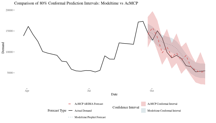
AcMCP, for the cost of increased complexity and computation, does give us confidence intervals that are more adaptive and ensure coverage into the uncertain future. However, it is not clear (to me, yet) how one could incorporate this into a production workflow to make actual online conformal predictions and keep track of them over time.

Addendum: univariate financial time series

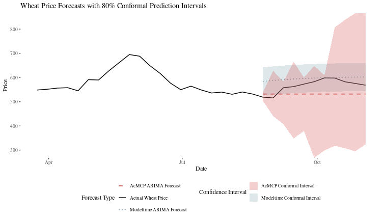
For completeness, we will look at time series which are unlikely to have the strong seasonality of the synthetic data we examioned above. In particular, we will pull daily prices for wheat, urea and oil from yahoo, and smooth them to get weekly average prices. Then, we will forecast wheat prices with urea and oil as exogenous data, using both modeltime-arima and acmcp-arima.

Pulling and preparing the data

library(tidyverse)
library(quantmod)
library(forecast)
library(zoo)
library(lubridate)
library(ggthemes)
library(scales)

commodity_tickers <- tibble(
  symbol = c("ZW=F", "CL=F", "UAN"),
  name = c("Wheat", "Oil", "Urea")
)

fetch_single_commodity <- function(symbol, name, start_date, end_date) {
  result <- try({
    getSymbols(symbol, src = "yahoo", 
               from = start_date, 
               to = end_date, 
               auto.assign = FALSE) |>
      as_tibble(rownames = "date") |>
      select(date, adjusted = ends_with("Adjusted")) |>
      rename_with(~ name, matches("adjusted"))
  }, silent = TRUE)

  if (inherits(result, "try-error")) {
    warning(str_glue("Error fetching {name}: {result}"))
    return(NULL)
  }

  result
}

interpolate_series <- function(x) {
  if (all(is.na(x))) return(x)
  ts_data <- ts(x, frequency = 7)
  na.interp(ts_data) |>
    as.numeric()
}

get_commodity_prices <- function(years_back = 5) {
  end_date <- today()
  start_date <- end_date - years(years_back)

  price_data <- commodity_tickers |>
    mutate(
      data = map2(
        symbol, name,
        ~fetch_single_commodity(.x, .y, start_date, end_date)
      )
    ) |>
    pull(data) |>
    reduce(full_join, by = "date")
  price_data |>
    mutate(
      date = ymd(date),
      across(-date, interpolate_series)
    ) |>
    as_tibble() |>
    structure(
      data_source = "Yahoo Finance",
      last_updated = now(),
      years_covered = years_back
    )
}

get_weekly_prices <- function(daily_prices) {
  daily_prices |>
    mutate(
      Week_Ending = case_when(
        wday(date, week_start = 1) == 6 ~ date,
        TRUE ~ date + days(7 - wday(date, week_start = 1))
      )
    ) |>
    group_by(Week_Ending) |>
    summarise(
      across(-date, ~mean(., na.rm = TRUE))
    ) |>
    filter(
      if_any(-Week_Ending, ~!is.na(.))
    ) |>
    arrange(Week_Ending) |> 
    mutate(date = Week_Ending) |> 
    select(-Week_Ending)
}

plot_commodity_prices <- function(df) {
  df |>
    pivot_longer(
      -date, 
      names_to = "Commodity", 
      values_to = "Price"
    ) |>
    ggplot(aes(x = date, y = Price)) +
    geom_line(aes(color = Commodity)) +
    facet_wrap(~Commodity, scales = "free_y", ncol = 1) +
    scale_color_manual(
      values = c("#8b1a1a", "#4a5568", "#6b6b6b")
    ) +
    theme_tufte() +
    labs(
      title = "Commodity Prices Over Time",
      x = NULL,
      y = "Price"
    )
}

prices <- get_commodity_prices(years_back = 5)
weekly_prices <- prices |> get_weekly_prices()

weekly_prices |>
  plot_commodity_prices() +
  labs(title = "Weekly Average Commodity Prices")

center

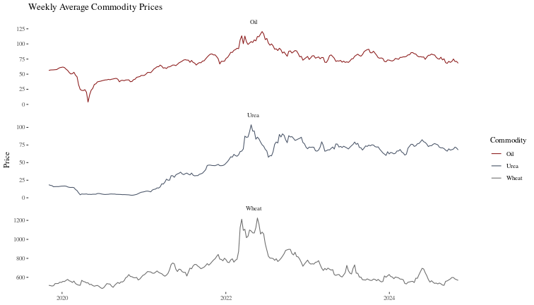
Then, we build simple models for the exogenous variables and prepare the data so that our forecasts for wheat are ex-ante.

data_split <- initial_time_split(weekly_prices, prop = holdout_prop)
train_set <- training(data_split)
holdout <- testing(data_split)
cal_set <- initial_time_split(holdout, prop = holdout_prop) |> training()
test_set <- initial_time_split(holdout, prop = holdout_prop) |> testing()

oil_model <- arima_reg() |> 
  set_engine(engine = "auto_arima") |>  
  fit(Oil ~ date, data = train_set)

urea_model <- arima_reg() |> 
  set_engine(engine = "auto_arima") |> 
  fit(Urea ~ date, data = train_set)

oil_model_tbl <- modeltime_table(oil_model)
urea_model_tbl <- modeltime_table(urea_model)

oil_forecast_tbl <- oil_model_tbl |> 
  modeltime_forecast(new_data = holdout, actual_data = weekly_prices)

urea_forecast_tbl <- urea_model_tbl |> 
  modeltime_forecast(new_data = holdout, actual_data = weekly_prices)

holdout$Oil <- {oil_forecast_tbl |> filter(.key == "prediction")}$.value
holdout$Urea <- {urea_forecast_tbl |> filter(.key == "prediction")}$.value

cal_set <- initial_time_split(holdout, prop = holdout_prop) |> training()
test_set <- initial_time_split(holdout, prop = holdout_prop) |> testing()
data_exante <- bind_rows(train_set, holdout)

Modeltime forecast for wheat

wheat_model <- arima_reg() |> 
  set_engine(engine = "auto_arima") |> 
  fit(Wheat ~ date + Oil + Urea, data = train_set)

model_tbl <- modeltime_table(wheat_model)

calibration_tbl <- model_tbl |> 
  modeltime_calibrate(new_data = cal_set, quiet = FALSE)

forecast_tbl <- calibration_tbl |> 
  modeltime_forecast(
    new_data = test_set, 
    actual_data = data_exante,
    conf_method = "conformal_default", 
    conf_interval = level_conf, 
    keep_data = TRUE
  )

Now, as before, the AcMCP forecast for wheat.

horizon <- nrow(test_set)

wheat_forecast <- function(y, h, level, xreg, newxreg) {
    model <- auto.arima(y, xreg = xreg)
    fc <- forecast(model, h = h, xreg = newxreg, level = level)
    return(fc)
}

xreg_matrix <- cbind(
  Oil = data_exante$Oil,
  Urea = data_exante$Urea
) |> head(nrow(train_set) + nrow(cal_set) + horizon)

wheat_fc <- cvforecast(
    y = ts({rbind(train_set, cal_set) |> select(Wheat)}, frequency = 52),
    forecastfun = wheat_forecast,
    h = horizon,
    level = c(level_conf),
    xreg = xreg_matrix,
    initial = 10, 
    window = horizon*10
)

cal_window <- max(10, horizon*5)
symm <- FALSE
roll <- FALSE
Tg <- 4
delta <- 0.01
Csat <- 2 / pi * (ceiling(log(Tg) * delta) - 1 / log(Tg))
KI <- 0.5
lr <- 0.1

acmcp <- mcp(wheat_fc, 
             alpha = 1 - 0.01 * wheat_fc$level,
             ncal = cal_window, 
             rolling = roll,
             integrate = TRUE, 
             scorecast = TRUE,
             lr = lr, 
             KI = KI, 
             Csat = Csat)

Now, we will prepare the data to compare the two conformal forecasts.

acmcp_df <- tibble(
  date = {head(data_exante$date, {nrow(train_set) + nrow(cal_set) + horizon}) |> tail(horizon)}, 
  acmcp_lower = acmcp$lower,
  acmcp_upper = acmcp$upper,
  acmcp_forecast = acmcp$mean
)

forecast_comparison_df <- forecast_tbl |>
  filter(.key %in% c("prediction")) |>
  select(date, .value, .conf_lo, .conf_hi, Wheat) |>
  rename(
    Wheat = Wheat,
    modeltime_forecast = .value,
    modeltime_lower = .conf_lo,
    modeltime_upper = .conf_hi
  ) |>
  right_join(acmcp_df, by = "date")  

forecast_comparison_df_2 <- bind_rows(
  train_set, 
  cal_set, 
  forecast_comparison_df
) |> 
  tail(horizon*3)

ggplot(forecast_comparison_df_2, aes(x = date)) +
  geom_line(aes(y = Wheat, color = "Actual Wheat Price"), size = 0.7) +
  geom_line(aes(y = modeltime_forecast, color = "Modeltime ARIMA Forecast"), 
            linetype = "dotted", size = 0.7) +
  geom_ribbon(aes(ymin = modeltime_lower, ymax = modeltime_upper, 
                  fill = "Modeltime Conformal Interval"), alpha = 0.2) +
  geom_line(aes(y = acmcp_forecast, color = "AcMCP ARIMA Forecast"), 
            linetype = "dashed", size = 0.9) +
  geom_ribbon(aes(ymin = acmcp_lower, ymax = acmcp_upper, 
                  fill = "AcMCP Conformal Interval"), alpha = 0.3) +
  scale_color_manual(
    values = c(
      "Actual Wheat Price" = "black","Modeltime ARIMA Forecast" = "#5A8D9B", "AcMCP ARIMA Forecast" = "#D95F5F"
    )
  ) +
  scale_fill_manual(
    values = c(
      "Modeltime Conformal Interval" = "#5A8D9B", "AcMCP Conformal Interval" = "#D95F5F"
    )
  ) +
  labs(
    title = "Wheat Price Forecasts with 80% Conformal Prediction Intervals",
    y = "Price",
    x = "Date",
    fill = "Confidence Interval",
    color = "Forecast Type"
  ) +
  theme_tufte(base_size = 12) +
  theme(
    legend.position = "bottom"
  ) +
  guides(
    color = guide_legend(nrow = 3),
    fill = guide_legend(nrow = 2)
  )

center

p. bhogale

Generating simple time series data

The modeltime workflow for time series forecasting

Split Conformal Inference in Time Series

Recipe for Split Conformal Prediction

Horizon-Dependent Quantiles

Online Conformal Inference for Multi-step Time Series Predictions

The AcMCP (Autocorrelated Multi-step Conformal Prediction) Method

Addendum: univariate financial time series

Pulling and preparing the data

The `modeltime` workflow for time series forecasting