 p. bhogale
 These notes are meant to implement little examples from Francois Fleuret's Little Book of Deep Learning (pdf link) in r-torch. I'm writing these as a fun way to dive into torch in R while surveying DL quickly.
You'll need to have the book with you to understand these notes, but since it is available freely, that ought not to be an issue.
Basis function regression
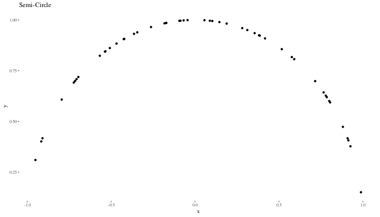
We will generate synthetic data that is similar to the example shown in the book:
# Number of samples
n <- 50

# Randomly distributed x values from -1 to 1
set.seed(123) # for reproducibility
x <- runif(n, min = -1, max = 1)
x <- sort(x) # Sorting for plotting purposes

# y values as the semi-circle
y <- sqrt(1 - x^2)

# Plotting the original semi-circle with randomly distributed x
data <- data.frame(x = x, y = y)
ggplot(data, aes(x, y)) +
  geom_point() +
  theme(element_text(size = 30)) +
  ggtitle("Semi-Circle") +
  theme_tufte()
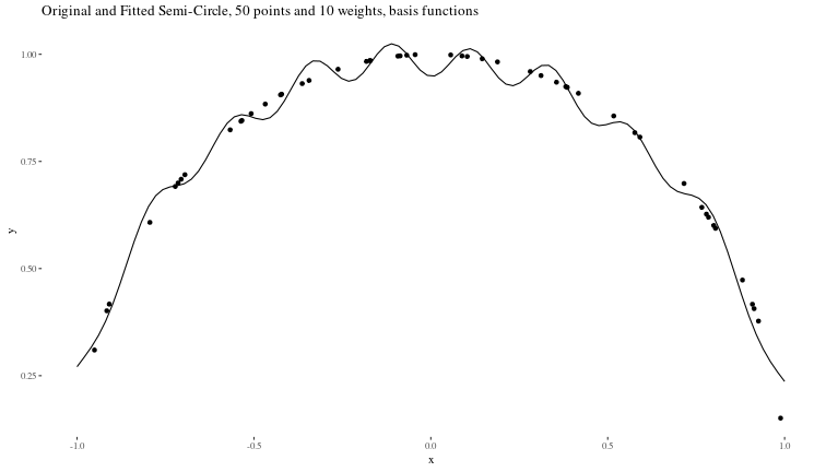
Following the book, we use gaussian kernels as the basis functions to fit \(y \sim f(x;w)\), where \(w\) are the weights of the basis functions.
# Define Gaussian basis functions
basis_functions <- function(x, centers, scale = 0.1) {
  exp(-((x - centers)^2) / (2 * scale^2))
}

# Centers of the Gaussian kernels, these do cover the region of space we are interested in
centers <- seq(-1, 1, length.out = 10)
Now, we define our model for \(y\), which, for basis function regression, is a linear combination of the basis functions initialized with random weights \(w\).
# Initial random weights
weightss <- torch_randn(length(centers), requires_grad = TRUE)

# Calculate the model output
model_y <- function(x) {
  # Convert x to a torch tensor if it isn't already one
  x_tensor <- torch_tensor(x)

  # Create a tensor for the basis functions evaluated at each x
  # Resulting tensor will have size [length(x), length(centers)]
  basis_matrix <- torch_stack(lapply(centers, function(c) basis_functions(x_tensor, c)), dim = 2)

  # Calculate the output using matrix multiplication
  # basis_matrix is [n, 10] and weights is [10, 1]
  y_pred <- torch_matmul(basis_matrix, weightss)

  # Flatten the output to match the dimension of y
  return(y_pred)
}
Now,we will use gradient descent to minimise the MSE between the model and the real values of \(y\) to obtain the optimal weights \(w^*\).
# Learning rate
lr <- 0.01

# Gradient descent loop
for (epoch in 1:5000) {
  y_pred <- model_y(x)

  op <- nnf_mse_loss(y_pred, torch_tensor(y))

  # Backpropagation
  op$backward()

  # Update weights
  with_no_grad({
    weightss$sub_(lr * weightss$grad)
    weightss$grad$zero_()
  })
}
Now, we can see how good our predictions are:
# Get model predictions
fin_x <- seq(-1,1,length.out=100)
final_y <- model_y(fin_x)

# Plotting
predicted_data <- data.frame(x = fin_x, y = as.numeric(final_y))
ggplot() +
  geom_point(data = data, aes(x, y)) +
  geom_line(data = predicted_data, aes(x, y)) +
  theme(element_text(size = 30)) +
  ggtitle("Original and Fitted Semi-Circle, 50 points and 10 weights, basis functions") +
  theme_tufte()
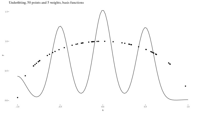
Underfitting When the model is too small to capture the features of the data (in our case, too few weights)
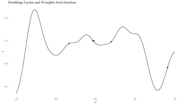
Overfitting When there is too little data to properly constrain the parameters of a larger model.
Classification, and the usefulness of depth
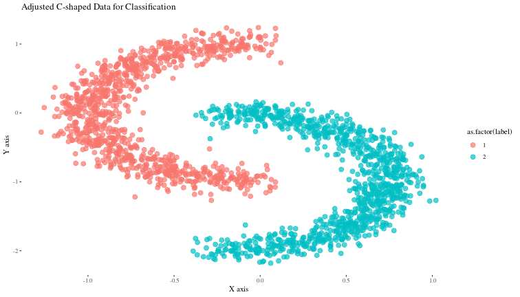
Let us generate data that looks similar to that shown in section 3.5 of the book.
# Function to generate C-shaped data
generate_c_data <- function(n, x_offset, y_offset, y_scale, label, xflipaxis) {
  theta <- runif(n, pi/2, 3*pi/2)  # Angle for C shape
  x <- cos(theta) + rnorm(n, mean = 0, sd = 0.1) + x_offset
  if(xflipaxis==T){
    x <- 1-x
  }
  y <- sin(theta) * y_scale + rnorm(n, mean = 0, sd = 0.1) + y_offset
  data.frame(x = x, y = y, label = label)
}

# Number of points per class
n_points <- 1000

# Generate data for both classes
data_class_1 <- generate_c_data(n_points, x_offset = 0,
                                y_offset = 0, y_scale = 1, label = 1,
                                xflipaxis = F)
data_class_0 <- generate_c_data(n_points, x_offset = 1.25,
                                y_offset = -1.0, y_scale = -1, label = 2,
                                xflipaxis = T)  # Mirrored and adjusted

# Combine data
data <- rbind(data_class_0, data_class_1)

# Plotting the data
ggplot(data, aes(x, y, color = as.factor(label))) +
  geom_point(alpha = 0.7, size = 3) +
  theme(element_text(size = 30)) +
  labs(title = "Adjusted C-shaped Data for Classification", x = "X axis", y = "Y axis") +
  theme_tufte()
Now, we can build a very simple neural net to classify these points and try to visualize what the trained net is doing at each layer.
net <- nn_module(
  "ClassifierNet",
  initialize = function() {
    self$layer1 <- nn_linear(2, 2)
    self$layer2 <- nn_linear(2, 2)
    self$layer3 <- nn_linear(2, 2)
    self$layer4 <- nn_linear(2, 2)
    self$layer5 <- nn_linear(2, 2)
    self$layer6 <- nn_linear(2, 2)
    self$layer7 <- nn_linear(2, 2)
    self$output <- nn_softmax(2)
    # Initialize an environment to store activations
    self$activations <- list()
  },

  forward = function(x) {
    x <- self$layer1(x) |> tanh()
    self$activations$layer1 <- x
    x <- self$layer2(x) |> tanh()
    self$activations$layer2 <- x
    x <- self$layer3(x) |> tanh()
    self$activations$layer3 <- x
    x <- self$layer4(x) |> tanh()
    self$activations$layer4 <- x
    x <- self$layer5(x) |> tanh()
    self$activations$layer5 <- x
    x <- self$layer6(x) |> tanh()
    self$activations$layer6 <- x
    x <- self$layer7(x) |> tanh()
    self$activations$layer7 <- x
    x <- self$output(x)
    x
  }
)

# Convert the features and labels into tensors
features <- torch_tensor(as.matrix(data[c("x", "y")]))
labels <- torch_tensor(as.integer(data$label))

# Create a dataset using lists of features and labels
data_classif <- tensor_dataset(features, labels)

# Create a dataloader from the dataset
dataloaders <- dataloader(data_classif, batch_size = 100, shuffle = TRUE)

# defining the model
model <- net |>
  setup(
    loss = nn_cross_entropy_loss(),
    optimizer = optim_adam
  ) |>
  fit(dataloaders, epochs = 50)
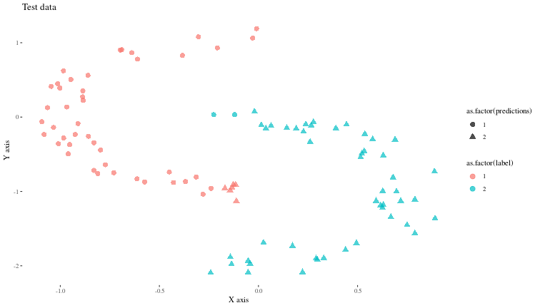
Now, let us see (visually) how well the model predicts some new synthetic data generated similarly.
# Number of points per class
n_points <- 50

# Generate data for both classes
test_data_class_1 <- generate_c_data(n_points, x_offset = 0,
                                y_offset = 0, y_scale = 1, label = 1,
                                xflipaxis = F)
test_data_class_0 <- generate_c_data(n_points, x_offset = 1.25,
                                y_offset = -1.0, y_scale = -1, label = 2,
                                xflipaxis = T)  # Mirrored and adjusted
# Combine data
test_data <- rbind(test_data_class_0, test_data_class_1)

# Convert the features and labels into tensors
test_features <- torch_tensor(as.matrix(test_data[c("x", "y")]))
test_labels <- torch_tensor(as.integer(test_data$label))

# Create a dataset using lists of features and labels
test_data_classif <- tensor_dataset(test_features, test_labels)

preds <- predict(model, test_data_classif) |>
  as.matrix()
colnames(preds) <- c("1","2")

predicted_labels <- apply(preds, 1, which.max)
test_data$predictions <- predicted_labels

# Plotting the data
ggplot(test_data, aes(x, y, color = as.factor(label), shape = as.factor(predictions))) +
  geom_point(alpha = 0.7, size = 3) +
  theme(element_text(size = 30)) +
  labs(title = "Test data", x = "X axis", y = "Y axis") +
  theme_tufte()
The activations for the forward model are stored in model$model$activations.
plots <- list()
test_data$label <- test_data$label |> as.factor()
plots[[1]] <- ggplot(test_data) +
  geom_point(aes(x, y, colour = label), alpha = 0.5) +
  labs(title = "Original", x = "X", y = "Y") +
  theme(aspect.ratio = 1) +
  theme_tufte()

# do a forward pass on the points
Y_temp <- model$model$forward(test_features)

num_layers <- model$model$activations |> length()
for (i in 1:num_layers) {
  df_temp <- model$model$activations[[i]] |> as.matrix() |> as_tibble()
  df_temp$label <- test_data$label
  plots[[i+1]] <- ggplot(df_temp) +
    geom_point(aes(x = V1, y = V2, colour = label), alpha = 0.5) +
    labs(title = paste("Layer ", i), x = "X", y = "Y") +
    theme(aspect.ratio = 1) +
    theme_tufte()
}
patchwork::wrap_plots(plots, ncol = 3)
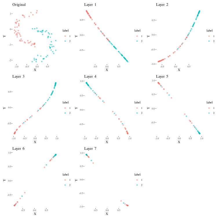
We can see how the linear layers modify space so that the points which are initially in interlocking C shapes become spatially seperated each subsequent layer.
Architectures
Multi Layer Perceptrons
This is a neural net that has a series of fully connected layers seperated by activations. We will illustrate an MLP using the Penguins dataset, where we try to predict the species of a penguin from some features. Example adapted from the excellent Deep Learning with R Torch book.
library(palmerpenguins)

penguins <- na.omit(penguins)
ds <- tensor_dataset(
  torch_tensor(as.matrix(penguins[, 3:6])),
  torch_tensor(
    as.integer(penguins$species)
  )$to(torch_long())
)

n_class <- penguins$species |> unique() |> length() |> as.numeric()
Now, we train a simple MLP on 75% of this dataset.
mlpnet <- nn_module(
  "MLPnet",
  initialize = function(din, dhidden1, dhidden2, dhidden3, n_class) {
    self$net <- nn_sequential(
      nn_linear(din, dhidden1),
      nn_relu(),
      nn_linear(dhidden1, dhidden2),
      nn_relu(),
      nn_linear(dhidden2, dhidden3),
      nn_relu(),
      nn_linear(dhidden3, n_class)
    )
  },
  forward = function(x) {
    self$net(x)
  }
)

total_size <- length(ds)
train_size <- floor(0.8 * total_size)
valid_size <- total_size - train_size

# Generate indices and shuffle them
set.seed(123)  # For reproducibility
indices <- sample(total_size)

train_indices <- indices[1:train_size]
valid_indices <- indices[(train_size + 1):total_size]

train_dataset <- ds[train_indices]
valid_dataset <- ds[valid_indices]

fitted_mlp <- mlpnet |>
  setup(loss = nn_cross_entropy_loss(), optimizer = optim_adam) |>
  set_hparams(din = 4,
              dhidden1 = 2,
              dhidden2 = 2,
              dhidden3 = 2,
              n_class = n_class) |>
  fit(train_dataset, epochs = 15, valid_data = valid_dataset)
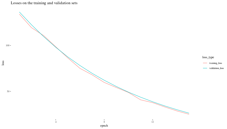
Now, let us visualize the validation loss during the training process.
fitted_mlp$records$metrics$train |>
  unlist() |>
  as_tibble()-> train_loss
colnames(train_loss) <- c("training_loss")
fitted_mlp$records$metrics$valid |>
  unlist() |>
  as_tibble()-> valid_loss
colnames(valid_loss) <- c("validation_loss")

loss_df <- cbind(train_loss, valid_loss) |>
  mutate(epoch = seq(1,nrow(train_loss))) |>
  pivot_longer(cols = c(training_loss, validation_loss),
               names_to = "loss_type",
               values_to = "loss")
ggplot(loss_df, aes(x = epoch, y = loss, colour = loss_type)) +
  geom_line() +
  theme(element_text(size = 30)) +
  theme_tufte() +
  labs(title = "Losses on the training and validation sets")
Convolutional networks - resnets
Images are usually dealt with by convolutional networks - they reduce the signal size until fully connected layers can handle it, or they output 2D signals which are themselves large. Residual networks involve an architecture where signal is taken from one layer and added to a later layer.
We will build a very simple resnet for the task of image classification, example loosely based on the DL+SC with R torch book.
library(torchvision)

set.seed(777)
torch_manual_seed(777)

dir <- "~/.torch-datasets"

train_ds <- torchvision::kmnist_dataset(train = TRUE,
  dir,
  download = TRUE,
  transform = function(x) {
    x |>
      transform_to_tensor()
  }
)
## Processing...
## Done!
valid_ds <- torchvision::kmnist_dataset(train = FALSE,
  dir,
  transform = function(x) {
    x |>
      transform_to_tensor()
  }
)

train_dl <- dataloader(train_ds,
  batch_size = 128,
  shuffle = TRUE
)
valid_dl <- dataloader(valid_ds, batch_size = 128)
There, we have downloaded the Kanji MNIST dataset to use to test our simple resnet. The model below is partially based on this tutorial from 2021.
# Define a simple Residual Block
simple_resblock <- nn_module(
  "SimpleResBlock",
  initialize = function(channels) {
    self$conv1 <- nn_conv2d(channels, channels, kernel_size = 3, padding = 1)
    self$relu1 <- nn_relu()
    self$conv2 <- nn_conv2d(channels, channels, kernel_size = 3, padding = 1)
    self$relu2 <- nn_relu()
  },
  forward = function(x) {
    identity <- x
    out <- self$relu1(self$conv1(x))
    out <- self$relu2(self$conv2(out))
    out + identity #the eponymous residual operation.
  }
)


net <- nn_module(
  "Net",

  initialize = function() {
    self$conv1 <- nn_conv2d(1, 32, 3, 1)
    self$conv2 <- nn_conv2d(32, 64, 3, 1)
    self$dropout1 <- nn_dropout(0.25)
    self$dropout2 <- nn_dropout(0.5)
    self$fc1 <- nn_linear(9216, 128)
    self$resblock1 <- simple_resblock(32) # 32 since its used after first conv layer that o/ps 32 channels
    self$resblock2 <- simple_resblock(64) # used after the second conv layer that outputs 64 channels
    self$fc2 <- nn_linear(128, 10)
  },

  forward = function(x) {
    x |>                                  # N * 1 * 28 * 28
      self$conv1() |>                     # N * 32 * 26 * 26
      nnf_relu() |>
      self$resblock1() |>                 # the residual block
      self$conv2() |>                     # N * 64 * 24 * 24
      nnf_relu() |>
      self$resblock2() |>                 # second residual block
      nnf_max_pool2d(2) |>                # N * 64 * 12 * 12
      self$dropout1() |>
      torch_flatten(start_dim = 2) |>     # N * 9216
      self$fc1() |>                       # N * 128
      nnf_relu() |>
      self$dropout2() |>
      self$fc2()                           # N * 10
  }
)
Now, we will train this on our data.
fitted <- net |>
  setup(
    loss = nn_cross_entropy_loss(),
    optimizer = optim_adam,
    metrics = list(
      luz_metric_accuracy()
    )
  ) |>
  fit(train_dl, epochs = 1)
Let's see how it does on the test set.
model_eval <- evaluate(fitted, valid_dl)
print(model_eval)
## A `luz_module_evaluation`
## ── Results ─────────────────────────────────────────────────────────────────────
## loss: 0.3452
## acc: 0.899
Attention and transformers
It seems to be a rule that any text on the internet mentioning these words must have this graphic from the original "Attention is all you need" paper.

Instead of the paper, read this excellent article by Sebastian Raschka. Transformers and Attention deserve a seperate article, but for now, it is worth mentioning that the inbuilt modules torch::nn_embedding and torch::nn_multihead_attention can be used to build out a simple transformer. Further topics mentioned in LBDL, the post above:
1. Causal self attention (nothing to do with causality in the Judea Pearl sense, just a condition on not letting tokens later in the sequence influence tokens that came before them).
2. Generative Pre-trained Transformer (GPT)
3. Vision transformer
Applications
Some simple example code based on the topics mentioned in the little book of deep learning.
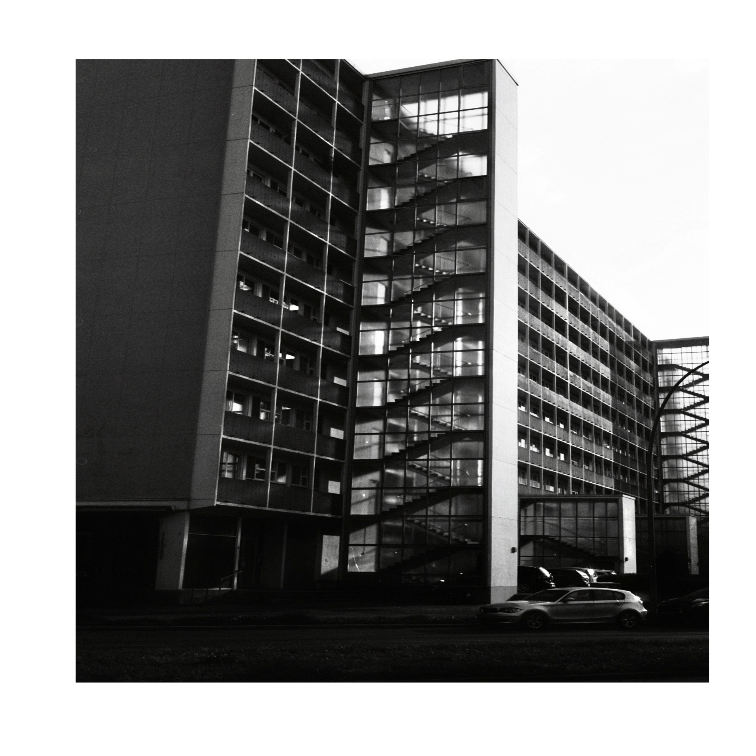
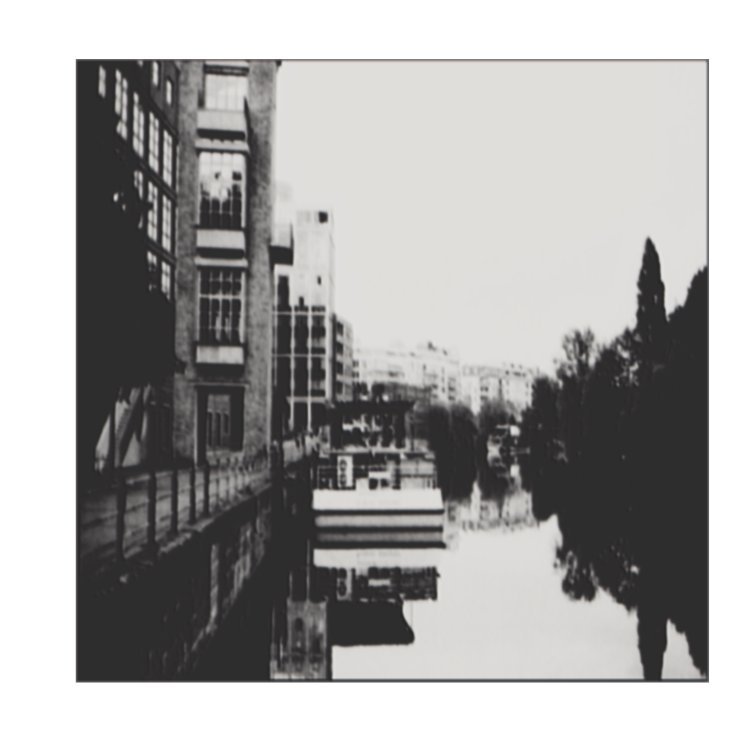
Image denoising
First, we want to generate some noisy images, we use some sample images. First, we would like to load and see these images in memory.
image_dir <- "./sample_photos/"
image_files <- list.files(image_dir, pattern = "\\.jpg$", full.names = TRUE)
images <- lapply(image_files, image_read)

# Determine maximum dimensions
max_width <- max(sapply(images, function(x) image_info(x)$width))
max_height <- max(sapply(images, function(x) image_info(x)$height))

# Pad and resize images
padded_images <- lapply(images, function(img) {
  image_background(image_resize(img, paste(max_width, 'x', max_height, '!')), "white")
})

# Function to properly convert ImageMagick image data to a torch tensor
padded_tensors <- lapply(padded_images, function(img) {
  # Extract pixel data as array
  array <- as.integer(image_data(img))
  # Convert the array to a tensor and normalize it
  tensor <- torch::torch_tensor(array, dtype = torch_float32()) / 255
  # Permute dimensions to have channel as the first dimension (if needed)
  tensor <- tensor$permute(c(3, 1, 2))
  return(tensor)
})


# Function to add random noise to an image tensor
add_noise_to_image <- function(image_tensor, noise_level = 0.1) {
  # Generate noise
  noise <- torch_rand_like(image_tensor) * noise_level
  # Add noise to the image
  noisy_image <- image_tensor + noise
  # Ensure the noisy image is still within the valid range [0, 1] if normalized or [0, 255] if not
  # Assuming the image tensor is normalized between 0 and 1
  # noisy_image <- torch_clamp(noisy_image, min = 0, max = 1)
  return(noisy_image)
}

# Function to display a torch tensor as an image using magick
plot_tensor_as_image <- function(tensor) {
  tensor |> as.array() |> aperm(c(2,3,1)) |> magick::image_read() -> imgg
  imgg |> plot()
  # return(imgg)
}

# Plot the first tensor
plot_tensor_as_image(padded_tensors[[4]])
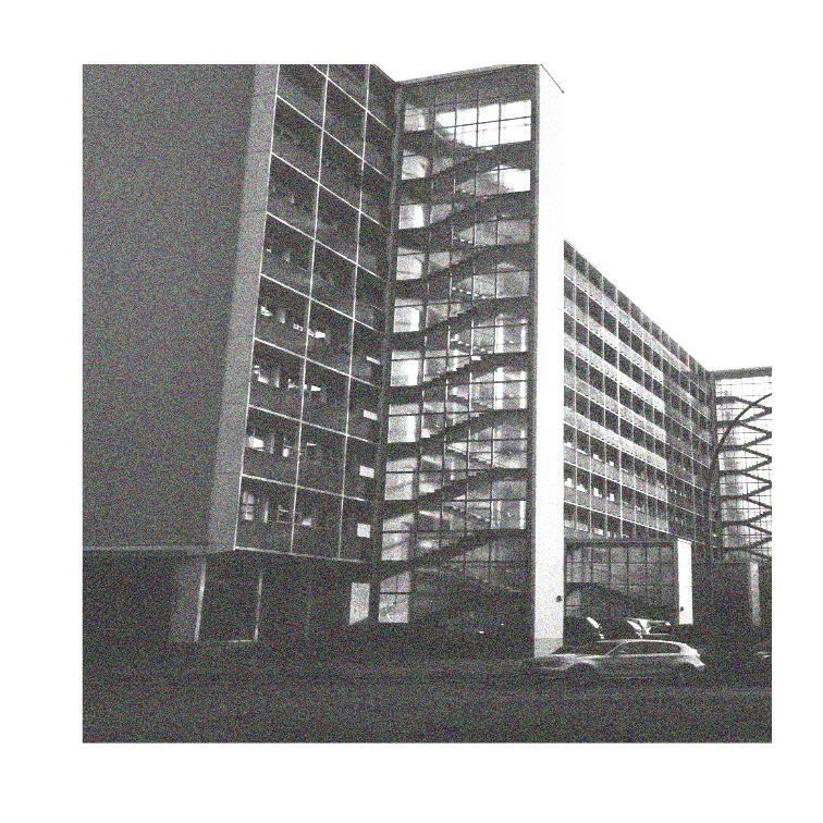
padded_tensors[[4]] |>
  add_noise_to_image(noise_level = 0.5) -> nimgg
plot_tensor_as_image(nimgg)
noisy_padded_tensors <- sapply(X = padded_tensors, FUN = add_noise_to_image, noise_level = 0.5)

# Now we will construct a dataset where the noisy images are inputs and the clean images are outputs.

# # Define the dataset
paired_dataset <- dataset(
  name = "PairedTensorDataset",
  initialize = function(inputs, targets) {
    self$x <- inputs
    self$y <- targets
  },
  .getitem = function(i) {
    list(input = self$x[[i]], target = self$y[[i]])
  },
  .length = function() {
    length(self$x)
  }
)

# Create an instance of the dataset
img_dat <- paired_dataset(noisy_padded_tensors, padded_tensors)

# Create a DataLoader
img_datlod <- dataloader(img_dat, batch_size = 1, shuffle = TRUE)
Now, we will train a very simple de-noising auto-encoder and test it on a new image. It will consist of a set of encoder layers that generate a compressed representation of the images and then decoder layers that will regenrate the originals back based on the copmopressed representation.
# Define the autoencoder model
autoencoder <- nn_module(
  "DenoisingAutoencoder",
  initialize = function() {
    # Encoder layers
    self$enc_conv1 <- nn_conv2d(in_channels = 3, out_channels = 4,
                                kernel_size = 7, stride = 1, padding = 0)
    self$enc_relu1 <- nn_relu()
    self$enc_conv2 <- nn_conv2d(in_channels = 4, out_channels = 2,
                                kernel_size = 7, stride = 1, padding = 0)
    self$enc_relu2 <- nn_relu()

    # Decoder layers
    self$dec_conv1 <- nn_conv_transpose2d(in_channels = 2, out_channels = 4,
                                          kernel_size = 7, stride = 1, padding = 0, output_padding = 0)
    self$dec_relu1 <- nn_relu()
    self$dec_conv2 <- nn_conv_transpose2d(in_channels = 4, out_channels = 3,
                                          kernel_size = 7, stride = 1, padding = 0, output_padding = 0)
    self$dec_sigmoid <- nn_sigmoid()
  },

  forward = function(x) {
    # Encoder
    x <- x |> # 3 1536 1560
      self$enc_conv1() |> # 4 1530 1554
      self$enc_relu1() |> # 4 1530 1554
      self$enc_conv2() |> # 2 1524 1548
      self$enc_relu2() # 2 1524 1548
    # Decoder
    x <- x |>
      self$dec_conv1() |> # 4 1530 1554
      self$dec_relu1() |> # 4 1530 1554
      self$dec_conv2() |> # 3 1536 1560
      self$dec_sigmoid() # 3 1536 1560
    x
  }
)

model_a <- autoencoder()
model_a$forward(noisy_padded_tensors[[1]]) |> dim()
## [1] 3 1536 1560
# Setup the model with luz
model_setup <- autoencoder |>
  setup(
    loss = nn_mse_loss(),
    optimizer = optim_adam,
    metrics = list(
      luz_metric_mse()
    )
  )

# Use the inbuilt learning rate finder
# rates_and_losses <- model_setup |>
#     lr_finder(img_datlod, start_lr = 0.0001, end_lr = 0.03)
# rates_and_losses |> plot()

# return_max_lr <- function(ral, threshfrac){
#     min_loss <- ral$loss |> min()
#     thresh <- min_loss * threshfrac
#     min_range <- min_loss - thresh
#     max_range <- min_loss + thresh
#     subset_df <- ral[ral$loss >= min_range & ral$loss <= max_range, ]
#     return(min(subset_df$lr))
# }
# print(return_max_lr(rates_and_losses, 0.05))
max_lr <- 0.0075 # return_max_lr(rates_and_losses, 0.05)

num_epochs <- 100

# fit the model and stop when improvements stop
fitted_model <- model_setup |>
    fit(img_datlod, epoch = num_epochs,
        valid_data = img_datlod,
        callbacks = list(
            luz_callback_early_stopping(
                monitor = "valid_loss",
                patience = 5,  # Number of epochs with no improvement after which training will be stopped
                min_delta = 0.001,  # Minimum change to qualify as an improvement
                mode = "min"  # 'min' mode means training will stop when the quantity monitored has stopped decreasing
                ),
            luz_callback_lr_scheduler(
                lr_one_cycle,
                max_lr = max_lr,
                epochs = num_epochs,
                steps_per_epoch = length(train_dl),
                call_on = "on_batch_end"
            )
            )
        )
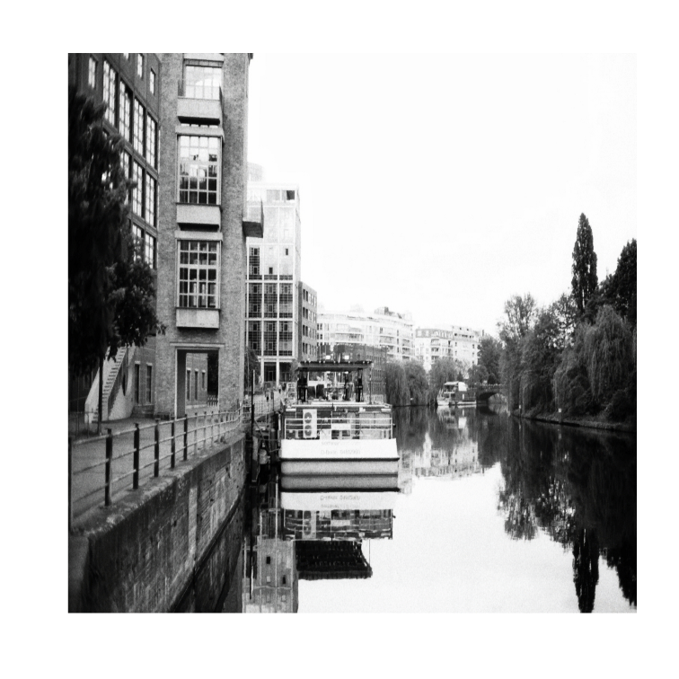
Now, let us see how the model does on the test photos. First, let us get the test images and add noise to them.
test_image_dir <- "./test_photos/"
test_image_files <- list.files(test_image_dir, pattern = "\\.jpg$", full.names = TRUE)
test_images <- lapply(test_image_files, image_read)
test_padded_images <- lapply(test_images, function(img) {
  image_background(image_resize(img, paste(max_width, 'x', max_height, '!')), "white")
})
test_padded_tensors <- lapply(test_padded_images, function(img) {
  # Extract pixel data as array
  array <- as.integer(image_data(img))
  # Convert the array to a tensor and normalize it
  tensor <- torch::torch_tensor(array, dtype = torch_float32()) / 255
  # Permute dimensions to have channel as the first dimension (if needed)
  tensor <- tensor$permute(c(3, 1, 2))
  return(tensor)
})
img_num <- 3
plot_tensor_as_image(test_padded_tensors[[img_num]])
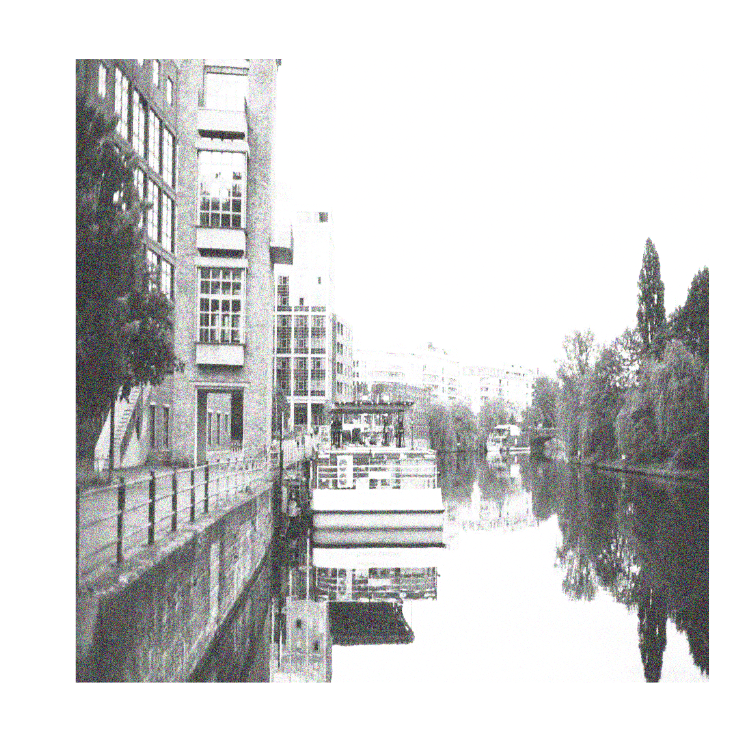
test_noisy_padded_tensors <- sapply(X = test_padded_tensors, FUN = add_noise_to_image, noise_level = 0.5)

test_padded_tensors[[img_num]] |>
  add_noise_to_image(noise_level = 0.5) -> test_nimgg
plot_tensor_as_image(test_nimgg)
test_img_dat <- paired_dataset(test_noisy_padded_tensors, test_padded_tensors)
test_img_datlod <- dataloader(test_img_dat, batch_size = 1, shuffle = TRUE)

fitted_model$model$forward(test_padded_tensors[[img_num]]) -> clean_test_nimgg
plot_tensor_as_image(clean_test_nimgg)
Even this small network trained on just 10 images is able to de-noise fairly well. Flavours of convolutional networks are used for some of the other applications mentioned in the book like:
- Object detection
- Semantic segmentation
On the other hand, encoder-decoder type architectures are used for applications like speech to text and image to text, where the encoder generates a representation of the speech or the image, and the decoder samples from text based on this representation after being trained.
Reinforcement learning algorithms train to maximize future reward by optimising a policy for choosing actions in the current state, under the markov assumption. The setup requires an "environemnt" that defines the states, rewards and actions possible in each state.
Diffusion based image generation is wild - first take images and slowly add noise until it is close to a simple normal or other analytical distribution, the image is gone. Train on these sequences and teach the network to de-noise, which means the network hallycinates images out of white noise. To have text influenced de-noising, try to decrease the distance between the text given and estimated image description by adding a bias to the denoising process.
Not covered in LBDL:
- RNNs
- GANs [TODO: this repo seems archived, so the code needs to be verified]
- VAEs [TODO: this repo seems archived, so the code needs to be verified]
- GNNs
- Self supervised learning