Reading material:

1. The tidy modeling book
2. The tidymodels blog on conformal regression
3. The notes of Angelopoulos
4. The notes of Tibshirani
5. The book of Christoph Molnar
6. The book of Valeriy Manokhin
7. The package of Sussman et al.

Getting some data

We will look at Indian trade data hosted on Kaggle for the purposes of illustrating tidy modeling techniques, without focusing too much on data exploration.

# pip install kaggle==1.6.14
# mkdir ~/.datasets/india_trade_data
# kaggle datasets download -d lakshyaag/india-trade-data
# mv india-trade-data.zip ~/.datasets/india_trade_data/
# unzip -d ~/.datasets/india_trade_data ~/.datasets/india_trade_data/india-trade-data.zip

read_csv("~/.datasets/india_trade_data/2010_2021_HS2_export.csv") -> df_hs2_exp

## Rows: 184755 Columns: 5
## ── Column specification ────────────────────────────────────────────────────────
## Delimiter: ","
## chr (3): HSCode, Commodity, country
## dbl (2): value, year
## 
## ℹ Use `spec()` to retrieve the full column specification for this data.
## ℹ Specify the column types or set `show_col_types = FALSE` to quiet this message.

read_csv("~/.datasets/india_trade_data/2010_2021_HS2_import.csv") -> df_hs2_imp

## Rows: 101051 Columns: 5
## ── Column specification ────────────────────────────────────────────────────────
## Delimiter: ","
## chr (3): HSCode, Commodity, country
## dbl (2): value, year
## 
## ℹ Use `spec()` to retrieve the full column specification for this data.
## ℹ Specify the column types or set `show_col_types = FALSE` to quiet this message.

df_hs2_exp |> mutate(trade_direction = "export") -> df_hs2_exp
df_hs2_imp |> mutate(trade_direction = "import") -> df_hs2_imp

df_hs2 <- bind_rows(list(df_hs2_exp, df_hs2_imp)) |> 
  mutate(value = case_when(
    is.na(value) ~ 0,
    TRUE ~ value
  ),
  year = as.integer(year),
  country = case_when(
    country == "U S A" ~ "United states of America",
    country == "U K" ~ "United Kingdom",
    TRUE ~ country
  ))

indicators <- c("gdp" = "NY.GDP.MKTP.CD", # GDP in current dollars
                "population" = "SP.POP.TOTL", # population
                "land_area" = "EN.LAND.TOTL" # total land
                )
WDI(indicator = indicators, start = 2010, end = 2021) -> wb_df

df_hs2 |> mutate(iso3c = country_name(x = country, to="ISO3")) -> df_hs2

## Some country IDs have no match in one or more of the requested country naming conventions, NA returned.
## Multiple country IDs have been matched to the same country name.
## There is low confidence on the matching of some country names, NA returned.
## 
## Set - verbose - to TRUE for more details

df <- left_join(df_hs2, wb_df, by = c("iso3c", "year")) |> 
  select(Commodity, value, country = country.y, year, trade_direction, iso3c, gdp, population) |> 
  group_by(country, year, trade_direction) |> 
  summarise(value = sum(value), gdp = gdp[1], population = population[1], .groups = "drop")

rm(df_exp, df_hs2, df_hs2_exp, df_hs2_imp, df_imp, wb_df)

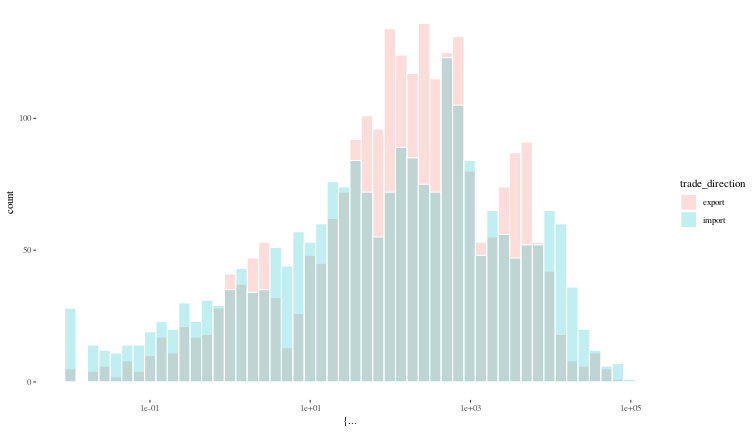
Just for simplicity, we will stick to the HS2 files (2010-2021), and ignore the other two (HS trade data) files that run from 2010-2018. We will combine the two files into a single data frame with an added column indicating direction of trade. We also interpret NAs in the value column to mean that there was no trade, and replace those with 0.

To make this something of a modelling challenge, we have enhanced the data with some information about the countries India is trading with, like the GDP. We downloaded GDP data from the World Bank with the WDI package. Then, we did a left join onto the Indian trade data on country and year, by first converting the countries in the Indian trade dataset to their ISO3 codes via the countries package.

The data frame we now have will serve as the basis for us to explore tidy modeling and conformal prediction in R.

df |> sample_n(10)

## # A tibble: 10 × 6
##    country        year trade_direction   value           gdp population
##    <chr>         <int> <chr>             <dbl>         <dbl>      <dbl>
##  1 Guinea         2010 import           103.     6853467832.   10270728
##  2 New Caledonia  2018 import             0.21   9896402284.     271170
##  3 Botswana       2014 import          1013.    15470088501.    2260376
##  4 Kuwait         2019 import          9574.   138696321088.    4441100
##  5 Pakistan       2016 export          1822.   313630000130.  213524840
##  6 Belize         2010 export            14.3    1739070295.     322106
##  7 Gambia, The    2014 import            36.1    1229461721.    2189019
##  8 Cuba           2020 export            20.3  107351800000    11300698
##  9 Puerto Rico    2012 export           106.   101564800000     3634488
## 10 Faroe Islands  2014 import             0.07   2914012679.      48465

ggplot({df |> na.omit()}, aes(x = {value}, fill = trade_direction)) +
  geom_histogram(bins = 50, col = "white", alpha = 0.25, position = "identity") +
  scale_x_log10() +
  theme_tufte()

Tidy modeling in R

Since the quantitative columns like value, gdp and population vary by orders of magnitude over the data, it probably makes sense to log transform them. To deal with 0 values, we add 1 to all the values, and omit rows which have any data missing. Now we split the data into training and test using built in functions from the rsample package, making sure that the distribution of the value column is similar in all our data splits using the strata argument.

set.seed(1)

trade_split <- initial_validation_split({df |> na.omit() |> mutate(year = as.factor(year), value = log(value+1))}, prop = c(0.6, 0.2), strata = value)
trade_split |> print()

## <Training/Validation/Testing/Total>
## <2856/952/952/4760>

train_df <- training(trade_split)
val_df <- validation(trade_split)
test_df <- testing(trade_split)


trade_simple_regression <- 
  recipe(value ~ ., data = {train_df |> 
      select(-country)}) |> 
  step_naomit() |> 
  step_log(gdp, population) |> 
  step_dummy(all_nominal_predictors()) |> 
  step_normalize(gdp, population)

Linear model

As a baseline, always best to begin with a simple, interpretable linear model.

linear_model <- linear_reg() |> 
  set_engine("lm") 

linear_workflow <- workflow() |>
  add_recipe(trade_simple_regression) |> 
  add_model(linear_model)

linear_fit <- fit(linear_workflow, train_df)

linear_fit |> tidy() |> arrange(p.value) |> head(5)

## # A tibble: 5 × 5
##   term                   estimate std.error statistic   p.value
##   <chr>                     <dbl>     <dbl>     <dbl>     <dbl>
## 1 (Intercept)               4.82     0.100      48.1  0        
## 2 gdp                       1.58     0.0463     34.1  5.37e-214
## 3 population                0.925    0.0463     20.0  2.49e- 83
## 4 trade_direction_import   -0.469    0.0545     -8.61 1.21e- 17
## 5 year_X2021                0.308    0.136       2.26 2.37e-  2

Now, let us make some predictions on the test data.

trade_reg_metrics <- metric_set(rmse, rsq, mae)
linear_test_preds <- predict(linear_fit, new_data = test_df) |> 
  bind_cols(test_df |> select(value))
# linear_val_preds |> head()
trade_reg_metrics(linear_test_preds, truth = value, estimate = .pred) |> 
  transmute(metric = .metric, linear_model_test = .estimate) -> linear_test_perf

Regression with XGBoost

We will now use the same modules of the parsnip package with XGBoost, since this is more likely to be used in production use-cases. Could hardly be easier.

xgb_model <- boost_tree(mtry = 3, trees = 5000, min_n = 7, tree_depth = 5, learn_rate = 0.01) |> 
  set_engine("xgboost") |> 
  set_mode("regression")

xgb_workflow <- workflow() |>
  add_recipe(trade_simple_regression) |> 
  add_model(xgb_model)

xgb_fit <- fit(xgb_workflow, train_df)

xgb_test_preds <- predict(xgb_fit, new_data = test_df) |> 
  bind_cols(test_df |> select(value))
trade_reg_metrics(xgb_test_preds, truth = value, estimate = .pred) |> 
  transmute(metric = .metric, xgb_model_test = .estimate) -> xgb_test_perf
left_join(linear_test_perf, xgb_test_perf)

## Joining with `by = join_by(metric)`

## # A tibble: 3 × 3
##   metric linear_model_test xgb_model_test
##   <chr>              <dbl>          <dbl>
## 1 rmse               1.49           1.17 
## 2 rsq                0.723          0.830
## 3 mae                1.12           0.858

XGB handily beats the linear model on test data.

Multiclass classification

Here, we will add back the country column and widen the data frame to show value of goods imported and exported by India with this country, and try to predict the country based on population, GDP, and trade with India.

spread(df, key = trade_direction, value = value) |> 
  na.omit() |> 
  mutate(country = as.factor(country)) |> 
  select(-year) -> df_classification

trade_class_split <- initial_validation_split(df_classification, prop = c(0.5,0.3), strata = country)

## Warning: Too little data to stratify.
## • Resampling will be unstratified.
## Too little data to stratify.
## • Resampling will be unstratified.

class_train_df <- training(trade_class_split)
class_test_df <- testing(trade_class_split)
class_val_df <- validation(trade_class_split)

trade_simple_classification <- 
  recipe(country ~ ., data = class_train_df) |> 
  step_naomit() |> 
  step_log(gdp, population) |> 
  step_normalize(all_numeric_predictors())

xgb_class_model <- boost_tree(mtry = 3, trees = 2000, min_n = 5, tree_depth = 5, learn_rate = 0.01) |> 
  set_engine("xgboost") |> 
  set_mode("classification")

xgb_class_workflow <- workflow() |>
  add_recipe(trade_simple_classification) |> 
  add_model(xgb_class_model)

xgb_class_fit <- fit(xgb_class_workflow, class_train_df)

xgb_class_test_preds <- predict(xgb_class_fit, new_data = class_test_df) |> 
  bind_cols(class_test_df |> select(country))
class_metrics <- metric_set(accuracy, mcc)
class_metrics(xgb_class_test_preds, truth = country, estimate = .pred_class) |> 
  transmute(metric = .metric, xgb_class_validation = .estimate) -> xgb_class_perf
xgb_class_perf

## # A tibble: 2 × 2
##   metric   xgb_class_validation
##   <chr>                   <dbl>
## 1 accuracy                0.448
## 2 mcc                     0.447

An accuracy of 40% for a messy classification problem with limited data and 208 classes is not too shabby at all, but adding any notion of confidence/coverage to a particular prediction is difficult (even if we have some kind of un-calibrated probability given by XGBoost), which is where conformal prediction comes in.

Conformal prediction

In what follows, we will follow the notation of Ryan Tibshirani (son of the redoubtable Rob Tibshirani), see the reading list above for a link to his notes.

Why conformal prediction

Machine learning models making point predictions do not reliably indicate how confident they are about those numbers, and even when we can get a confidence interval (for a linear regression), or a probability like score (for a classification), we cannot easily say (if at all) with what probability we will find the true value from an out of set data point in the confidence interval or the first few most probable values predicted by a classifier.

Very often, a decision about what to do and how to do it depends crucially on how sure we are of a prediction, and we would like very much to know how sure we can be that the true value falls within a certain finite range.

I see the Bayesians wildly waving their hands, and I'll confess my sins and say I identify as a Bayesian myself. However, the selection of priors for model parameters is a shaky business, and untenable in any careful artisanal way for a large black box model. Besides, Bayesian MCMC is computationally expensive and gets more so as the number of model parameters increase. Furthermore, getting a prediction distribution is expensive as we run the model forward drawing from the joint distribution of parameters to get an empirical distribution of predictions on which we can then make some probabilistic statements.

While Bayesian inference gives us a lot (especially if we are interested in knowing what part of the parameter space of a particular model of the world corresponds most closely to reality), it is rather overengineered and expensive in terms of effort and computation if all one wants is to attach interpretable uncertainty ranges to model predictions.

The field of conformal prediction - on the other hand - uses the notion of coverage and prediction bands, and the goal is to enhance point predictions with sets of predictions that are guaranteed (given all available data) to contain the true value with a certain probability.

Conformal basics - regression

If we have a set of \(n\) vectors each of \(d\) dimensions \(\{X_i\}\) (so \(X_i\) is in \(\mathbb{R}^d\)) where \(i \in [1,n]\), each of which is associated with an outcome \(Y_i\) in \(\mathbb{R}\), given a new prediction vector \(X_{n+1}\), we want to obtain a prediction band \(\hat{C}: X \rightarrow \{\text{subset of } \mathbb{R}\}\) such that we can guarantee that the probability of \(Y_{n+1}\) falling within the prediction band is greater than some threshold,

for a particular \(\alpha \in (0,1)\).

We - of course - would like the prediction bands to be narrower if its "easy" to predict the \(Y\)s from the \(X\)s, and we would like to do this with a finite data set and without much computation.

Surprisingly, this is plausible, under the assumption that the data (even the new data) are "exchangeable", which is to say that their joint distribution is invariant under permutations. This is a weaker assumption than the IID assumptions often made. Further more, our methods will not depend on the model parameters or reality having any specific distribution, which is a huge advantage over Bayesian techniques.

There are many ways to construct the prediction band, or to extend a point prediction to a prediction band, we will now discuss the simplest of these in the context of regression.

Split conformal prediction

First we note a basic property of a series of numbers \([Y_1, .., Y_n]\) drawn from some distribution. If another number \(Y_{n+1}\) is drawn from the same distribution,

which gives us a way to order a finite list of numbers such that another similar number has a certain probability \((1-\alpha)\) of falling within the first \(\lceil (1-\alpha)(n+1) \rceil\) numbers of that list. Thus, defining

gives us a one sided prediction interval \((-\infty, \hat{q}_n]\) where \(\mathbb{P}(Y_{n+1} \leq \hat{q}_n) \geq (1-\alpha)\). Using similar arguments to derive an upper bound, we have,

The recipe

We will now see how we can apply these inequalities to get some idea of uncertainty and coverage guarantees in regression problems.

1. Split the training set (\(n\) rows) into two sets:
   1. The proper training set \(D_1\) with \(n_1\) rows
   2. The calibration set \(D_2\) with \(n_2 = n-n_1\) rows
2. Train a point prediction model/function \(\hat{f}_{n_1}\) on \(D_1\).
3. Calculate the residuals \(R\) on the calibration set,
   $$R_i = |Y_i - \hat{f}_{n1}(X_i)|, \text{ }i \in D_2.$$
4. Calculate the conformal quantile \(\hat{q}_{n_2}\),
   $$\hat{q}_{n_2} = \lceil (1-\alpha)(n_2+1) \rceil \text{ smallest of } R_i, i \in D_2. $$
5. The, the desired prediction band is given by,
   $$\hat{C}_n(x) = [\hat{f}_{n_1} - \hat{q}_{n_2}, \hat{f}_{n_1} + \hat{q}_{n_2}],$$
   where we have a coverage guarantee,
   $$\mathbb{P}\left(Y_{n+1}\in\hat{C}_n(X_{n+1} | D_1)\right) \in \left[1-\alpha, 1-\alpha+\frac{1}{n_2+1} \right).$$

Note that there is nothing special about residuals, we can define any negatively oriented (smaller is better) conformity score \(V(D_2, \hat{f}_{n_1})\) that would work just as well to give a prediction band such that,

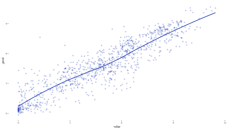
Now, we will revisit our initial regression problem and see what conformal prediction can do for us. This is what our xgboost model looks like when plotted against the test values.

ggplot({bind_cols({xgb_test_preds |> select(.pred)}, test_df)}) +
  geom_point(aes(x = value, y = .pred), alpha = 0.25, colour = "#2842b5") +
  geom_smooth(aes(x = value, y = .pred), alpha = 0.1, colour = "#2842b5", se = FALSE) +
  theme_tufte()

## `geom_smooth()` using method = 'loess' and formula = 'y ~ x'

Now, we will use the probably::int_conformal_split function to estimate the prediction bands at the 90% level, and we will use the validation set val_df that we have kept aside and never used as the calibration set for this.

split_con  <- int_conformal_split(xgb_fit, val_df)
test_split_result <- predict(split_con, test_df, level = 0.9) |> 
  bind_cols(test_df)

ggplot(test_split_result) +
  geom_point(aes(x = value, y = .pred), alpha = 0.25, colour = "#2842b5") +
  geom_smooth(aes(x = value, y = .pred_upper), colour = "#fcba03", se = FALSE) +
  geom_smooth(aes(x = value, y = .pred_lower), colour = "#fcba03", se = FALSE) +
  geom_smooth(aes(x = value, y = .pred), alpha = 0.1, colour = "#2842b5", se = FALSE) +
  theme_tufte()

## `geom_smooth()` using method = 'loess' and formula = 'y ~ x'
## `geom_smooth()` using method = 'loess' and formula = 'y ~ x'
## `geom_smooth()` using method = 'loess' and formula = 'y ~ x'

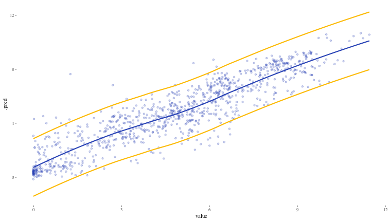
The interpretation of our prediction band within the framework of conformal prediction is that we would expect 90% (since that is the level we chose) of actual values to be within the interval computed based on our calibration set. Let us see how we do on coverage on our test set (we would expect it to be around 90%)

test_split_result |> 
  mutate(within_band = (.pred_lower <= value) & (value <= .pred_upper)) |> 
  summarise(coverage = mean(within_band) * 100)

## # A tibble: 1 × 1
##   coverage
##      <dbl>
## 1     92.3

Excellent.

While this is an encouraging result, there are clearly some improvements needed:

1. The prediction bands are based on the calibration set which was just 20% of the training set. If we use cross validation, we could get residuals for the entire training set and use those to calibrate the prediction bands.
2. The width of the prediction band seems constant through the entire range of values where as the points outside the range seem to occur (in this particular case) in the low and mid ranges. In general, it is reasonable to expect that the model will do better in some areas than in others, and the prediction band should reflect this, being wider in areas where the model is worse.

We now address the first point, and deal with the slightly more complex issue of adaptive conformal prediction in a subsequent section.

Split conformal prediction with CV

ctrl <- control_resamples(save_pred = TRUE, extract = I) # this line ensures out of sample preds are also stored in the CV process

trade_reg_folds <- vfold_cv({bind_rows(train_df, val_df)}, v = 10) # 10 fold CV

xgb_resample <- xgb_workflow |> 
  fit_resamples(trade_reg_folds, control = ctrl)

collect_metrics(xgb_resample)

## # A tibble: 2 × 6
##   .metric .estimator  mean     n std_err .config             
##   <chr>   <chr>      <dbl> <int>   <dbl> <chr>               
## 1 rmse    standard   1.16     10 0.0125  Preprocessor1_Model1
## 2 rsq     standard   0.829    10 0.00393 Preprocessor1_Model1

Now we again use the probably package to estimate the prediction band.

cv_con <- int_conformal_cv(xgb_resample)
test_cv_results <- predict(cv_con, test_df, level = 0.9) |> 
  bind_cols(test_df)

ggplot(test_cv_results) +
  geom_point(aes(x = value, y = .pred), alpha = 0.25, colour = "#2842b5") +
  geom_smooth(aes(x = value, y = .pred_upper), colour = "#fcba03", se = FALSE) +
  geom_smooth(aes(x = value, y = .pred_lower), colour = "#fcba03", se = FALSE) +
  geom_smooth(aes(x = value, y = .pred), alpha = 0.1, colour = "#2842b5", se = FALSE) +
  theme_tufte()

## `geom_smooth()` using method = 'loess' and formula = 'y ~ x'
## `geom_smooth()` using method = 'loess' and formula = 'y ~ x'
## `geom_smooth()` using method = 'loess' and formula = 'y ~ x'

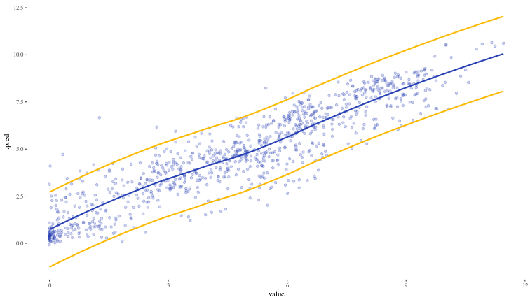
test_cv_results |> 
  mutate(within_band = (.pred_lower <= value) & (value <= .pred_upper)) |> 
  summarise(coverage = mean(within_band) * 100)

## # A tibble: 1 × 1
##   coverage
##      <dbl>
## 1     90.9

Full conformal prediction

Full conformal prediction is a delightfully simple and computationally impossible (except in some rare cases (that I have been assured do actually exist)) idea that is worth glancing at.

1. Use the entire training set (the proper training set as well as the calibration set are included) \(D_n = D_{1}\cup D_{2}\) such that \((X_i, Y_i) \in D_n\).
2. When there is a new predictor \(x \in \mathbb{R}^d\) available, evaluate a possible outcome \(y \in \mathbb{R}\) by training the model on \(D_n\) augmented with \((x,y)\), to get \(\hat{f}_{D_n\cup(x,y)}\), and calculating the residual \(R^{x,y} = |y - \hat{f}_{D_n\cup(x,y)}(x)|\).
3. We do this (augment the training set with one point \((x,y)\), and train the model on this, and calculate the residual) for all possible \(y\in \mathbb{R}\), and then define the prediction band to be,
   $$\hat{C}(x) = \left\{y: R^{(x,y)} \leq \lceil(1-\alpha)(n+1\rceil) \text{ smallest of } \underbrace{R_1, .. R_n}_{\text{training set residuals}} \right\}. $$
   Its clear that it is extremely computationally expensive (and hopelessly impractical) to search through the space of all possible \(y\) and to train the model on each one.

Keeping this aside, now, we address the second point raised earlier, that of adaptive prediction bands.

Adaptive conformal prediction

To obtain adaptive prediction bands, we use a method called Conformalized Quantile Regression (CQR). Usually (for example, when minimizing RMSE) we are estimating the expected value of the response variable given predictors. Quantile regression (see the package quantreg) tries to estimate a particular quantile \(\tau\) of the response variable instead of the mean, given some predictors. We denote a model estimating the \(\tau\) quantile of the outcome variable by \(\hat{f}^{\tau}_n\) where \(n\) is the number of examples in the training set.

CQR recipe

1. On the proper training set \(D_1\) with \(n_1\) examples as before, we train two quantile regression models \(\hat{f}^{\alpha/2}_{n_1}\) and \(\hat{f}^{1-\alpha/2}_{n_1}\). What we are doing here is just taking the upper and lower limits of the prediction band (remember, we define the prediction band by saying that we want to have a coverage probability of \((1-\alpha)\), which means everything below \(\alpha/2\) and everything above \(1-\alpha/2\) is excluded).
2. The calibration test scores are defined by,
   $$R_i = \text{max}\left[\hat{f}^{\alpha/2}_{n_1}(X_i)-Y_i, Y_i - \hat{f}^{1-\alpha/2}_{n_1}(X_i) \right], \text{ } i \in D_2.$$
3. As before, \(\hat{q}_{n_2} = \lceil (1-\alpha)(n_2+1) \rceil \text{ smallest of } R_i, i \in D_2\) , and the prediction band is given by,
   $$\hat{C}_n(x) = \left[ \hat{f}^{\alpha/2}_{n_1}(x) - \hat{q}_{n_2}, \hat{f}^{1-\alpha/2}_{n_1}(x)+\hat{q}_{n_2} \right].$$
   The adaptivity of the prediction interval comes the estimates of the quantiles by the quantile regression model.

Lets see an example of CQR in action using the probably package using the training and calibration sets, which uses quantile regression forests which are expected to be spectacularly bad for extrapolated data, but should do well otherwise.

cqr <- int_conformal_quantile(
  xgb_fit,
  train_data = train_df,
  cal_data = val_df,
  level = 0.9,
  ntree = 2200
)

test_cqr_results <- predict(cqr, test_df) |> 
  bind_cols(test_df)

ggplot(test_cqr_results) +
  geom_point(aes(x = value, y = .pred), alpha = 0.25, colour = "#2842b5") +
  geom_smooth(aes(x = value, y = .pred_upper), colour = "#fcba03", se = FALSE) +
  geom_smooth(aes(x = value, y = .pred_lower), colour = "#fcba03", se = FALSE) +
  geom_smooth(aes(x = value, y = .pred), alpha = 0.1, colour = "#2842b5", se = FALSE) +
  theme_tufte()

## `geom_smooth()` using method = 'loess' and formula = 'y ~ x'
## `geom_smooth()` using method = 'loess' and formula = 'y ~ x'
## `geom_smooth()` using method = 'loess' and formula = 'y ~ x'

test_cqr_results |> 
  mutate(within_band = (.pred_lower <= value) & (value <= .pred_upper)) |> 
  summarise(coverage = mean(within_band) * 100)

## # A tibble: 1 × 1
##   coverage
##      <dbl>
## 1     89.7

Honestly, for our data at least, that looks so much worse than just simple CV based split conformal prediction. Need to look into finding / implementing a better CQR method.

[TODO] Quantile regression with XGBoost and self implemented CQR scheme to see if that works better than this, also see/track these issues: quantile reg with rq in parsnip, quantile reg with xgb in parsnip.

Conformal basics - classification

For classification problems what we want is a set of classes that is guaranteed to include the true class with a certain probability. As such most schemes for conformal prediction on classification problems use the predicted probabilities given by the model.

Keeping the same notation as before, we assume that the model \(\hat{f}_{n_1}\) trained on the proper training set \(D_1\) gives us \(K\) probabilities, one for each of the \(K\) classes given the predictors \(x\).

We will outline a scheme called Adaptive Predictive Sets (APS).

1. For each example in the calibration set \(D_2\), calculate the conformity score as the sum of all probabilities greater than and including the probability assigned to the true class, which is to say we add up the probabilities of all classes which the model thought were at least as likely as the true class. This gives us the \(R_i, \text{ } i \in D_2\).
2. As before, we define \(\hat{q}_{n_2} = \lceil(1-\alpha)(n_2+1)\rceil\) smallest of the \(R_i, \text{ } i\in D_2\).
3. This gives us the prediction set, to be all classes (ordered in descending order of probability estimated by model) that need to be included for the sum of their probabilities to be at least \(\hat{q}_{n_2}\).

It looks like the probably package does not implement APS out of the box, so we will quickly do an implementation ourselves, following the recipe above.

# calculating the probability scores for validation set
xgb_class_val_preds <- predict(xgb_class_fit, new_data = class_val_df, type = 'prob') |> 
  bind_cols(class_val_df |> select(country))

# function that computes the conformity scores and using the alpha, returns the 
# quantile q on the basis of which prediction sets can be calculated
compute_conformity_scores <- function(data, alpha) {
  n_2 <- nrow(data)

  result <- data |> 
    rowwise() |> 
    mutate(
      p_i = get(paste0(".pred_", country))
    ) |>
    mutate(
      r_i = sum(c_across(starts_with(".pred_"))[c_across(starts_with(".pred_")) >= p_i])
    ) |> 
    ungroup() |> 
    select(conformity_score = r_i)

  q <- result |> 
    pull(conformity_score) |> 
    sort(decreasing = TRUE) |> 
    nth(ceiling((1 - alpha) * (n_2 + 1)) )

  list(conformity_scores = result, q = q)
}

compute_conformity_scores(xgb_class_val_preds, 0.7) -> conformity_scores
qn <- conformity_scores$q

# this function uses the probabilities returned by the model on the test data
# and uses the q computed by the function above to construct prediction sets
process_test_results <- function(test_data, q) {
  test_data |> 
    rowwise() |> 
    mutate(
      prediction_set = list({
        # Get all probability columns
        prob_cols <- grep("^\\.pred_", names(test_data), value = TRUE)

        # Create a named vector of probabilities
        probs <- c_across(starts_with(".pred_"))
        names(probs) <- prob_cols

        # Order probabilities in descending order
        sorted_probs <- sort(probs, decreasing = TRUE)

        # Sum probabilities until >= q
        cumsum_probs <- cumsum(sorted_probs)
        n_countries <- which(cumsum_probs >= q)[1]

        # Get country names for the summed probabilities
        country_names <- names(sorted_probs)[1:n_countries]

        # Remove ".pred_" prefix from country names
        str_remove(country_names, "^\\.pred_")
      })
    ) |> 
    ungroup() |> 
    select(prediction_set)
}

xgb_class_test_prob_preds <- predict(xgb_class_fit, new_data = class_test_df, type = 'prob') |> 
  bind_cols(class_test_df |> select(country))

process_test_results(xgb_class_test_prob_preds, qn) |> 
  bind_cols(class_test_df |> select(country)) |> 
  mutate(prediction_set_length = map_int(prediction_set, length)) -> prediction_set_sizes

prediction_set_sizes$prediction_set_length |> mean()

## [1] 19.10148

Now we can see how bad we are at predicting the country. Just to have a 70% guarantee of having the correct country in the set, we have a mean prediction set length of close to 20!

That concludes our romp through the basics of conformal prediction. We have not dealt with time series models and time series conformal prediction in this post.. next time.