 p. bhogale
 Disclaimer: statistics is hard - the chief skill seems to be the ability to avoid deluding oneself and others. This is something that is best and quickest learned via an apprenticeship in a group of careful thinkers trying to get things right. Tutorials like these can be misleading, in that they give the illusion of competence. This tutorial was written as a way for me to learn, not as an exposition by an experienced practitioner. However, I hope this serves as a useful read, expecially since I link to other, deeper resources.
If you want to peek into how a statistician thinking carefully approaches this subject, you could hardly do better than the Causal Mixtape and Statistical Rethinking. If you are totally new to all this causal stuff, do read The Book of Why (no, really).
This article heavily uses the quartets package and the paper that introduces it but there is also another paper(pdf) and associated package on a very similar theme. For analysing DAGs, we rely heavily on the wonderful dagitty package, and we visualize using ggdag.
The wind/rudder problem
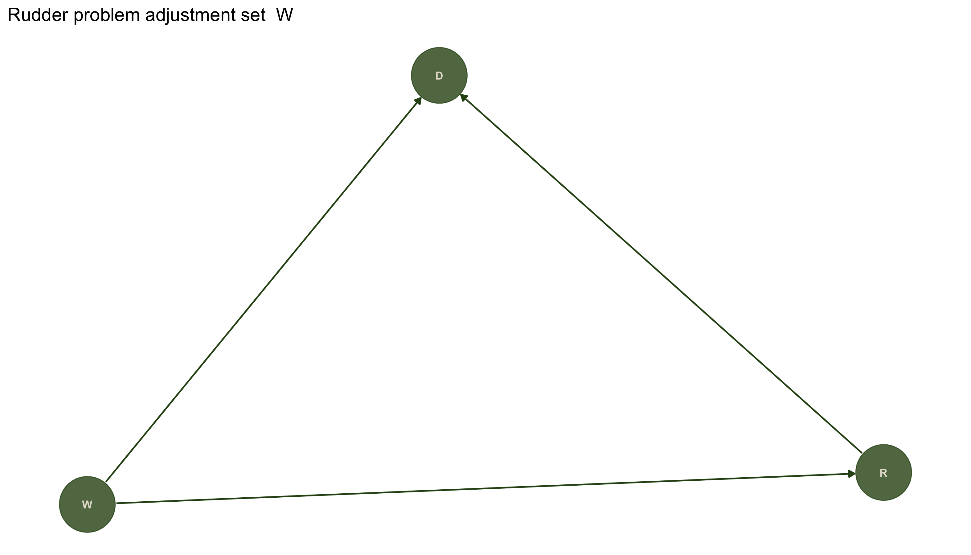
Consider a dynamic system consisting of three variables: wind speed \(W\), rudder angle \(R\), and boat heading \(D\) (direction). An observer on shore measures \(R\) and \(D\) continuously over time, with the goal of understanding whether rudder adjustments causally affect the boat's trajectory. The wind \(W\), however, remains unobserved.
The data-generating process works as follows. The wind \(W\) exerts a direct causal influence on the boat's heading: \(W \rightarrow D\). A skilled sailor observes the wind and adjusts the rudder to compensate, creating a second causal relationship: \(W \rightarrow R\). The rudder also directly affects heading through hydrodynamic forces: \(R \rightarrow D\). Crucially, the sailor's adjustment strategy is systematic: rudder angle is set to approximately counteract the wind's effect, meaning \(R \approx -\alpha W\) for some coefficient \(\alpha > 0\).
After collecting observational data, the observer computes \(\text{cor}(R, D)\) and finds it to be approximately zero. The naive conclusion follows: rudder angle has no relationship with boat direction, therefore the rudder is ineffective.
The error stems from endogeneity. In econometrics and causal inference, a variable is called endogenous when it is correlated with the error term or, equivalently, when it is determined by other variables in the system that also affect the outcome. Here, the rudder angle \(R\) is endogenous because it is not set independently of the other factors affecting direction, \(R\) is systematically determined by \(W\) (via the sailor working to keep the boat's heading constant), which is itself a common cause of both \(R\) and \(D\).
This creates what Pearl calls confounding: the naive correlation \(\text{cor}(R, D)\) confounds the true causal effect of \(R\) on \(D\) with the spurious correlation induced by their common cause \(W\). This and other seemingly intractable issues like Simpson's paradox (association between two variables changes sign when conditioned on a third) are all unravelled once we encode our knowledge of the world into causal relationships between variables and test how valid these are in light of data.
At the end of this article, you should be able to do a basic causal analysis on an appropriate dataset with dagitty and have an intuition about what it is you are saying when you estimate direct and indirect causal effects.
The data.
Let's load the causal quartet and take a first look. These four datasets were carefully constructed to have identical correlations between x and y, but as we'll discover, they tell four completely different causal stories.
## # A tibble: 10 × 6
## dataset exposure outcome covariate u1 u2
## <chr> <dbl> <dbl> <dbl> <dbl> <dbl>
## 1 (4) M-Bias 0.609 -0.0947 3.15 0.599 -0.739
## 2 (2) Confounder -0.849 -1.59 -0.282 NA NA
## 3 (2) Confounder -0.379 -1.05 -0.518 NA NA
## 4 (2) Confounder 2.44 2.94 0.654 NA NA
## 5 (2) Confounder -0.858 -0.802 -0.762 NA NA
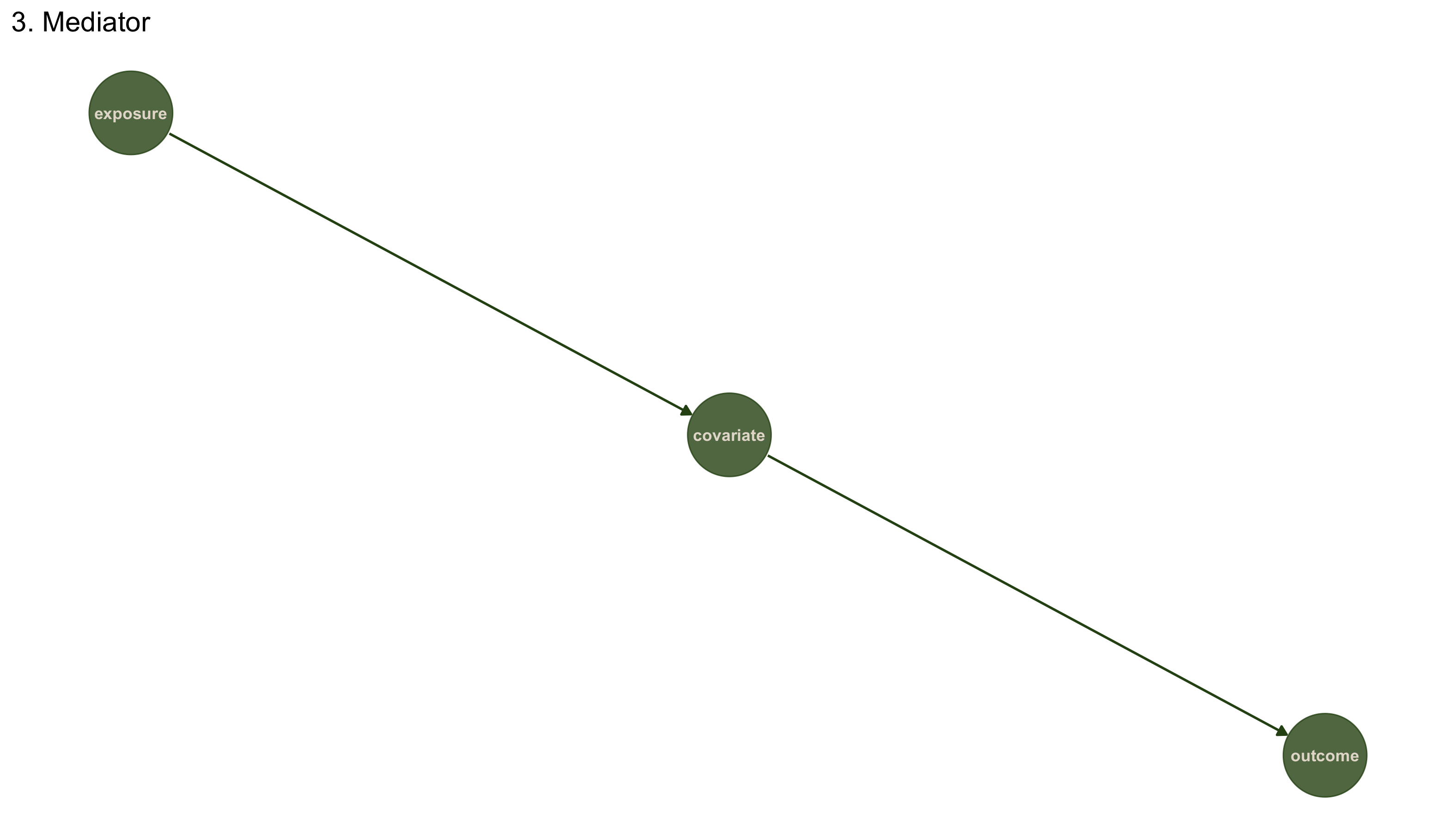
## 6 (3) Mediator 1.35 4.02 3.33 NA NA
## 7 (1) Collider -0.401 0.617 0.207 NA NA
## 8 (4) M-Bias -1.16 -2.51 -1.98 -0.124 -0.718
## 9 (2) Confounder 2.21 2.62 0.321 NA NA
## 10 (1) Collider -0.601 0.405 -0.303 NA NA
## # A tibble: 4 × 7
##   dataset            n  mean_x  mean_y  sd_x  sd_y cor_xy
##   <chr>          <int>   <dbl>   <dbl> <dbl> <dbl>  <dbl>
## 1 (1) Collider     100 -0.146  -0.0136  1.05  1.37  0.769
## 2 (2) Confounder   100 -0.0291 -0.0357  1.30  1.77  0.735
## 3 (3) Mediator     100 -0.0317 -0.0392  1.03  1.72  0.594
## 4 (4) M-Bias       100  0.136  -0.0809  1.48  2.06  0.724
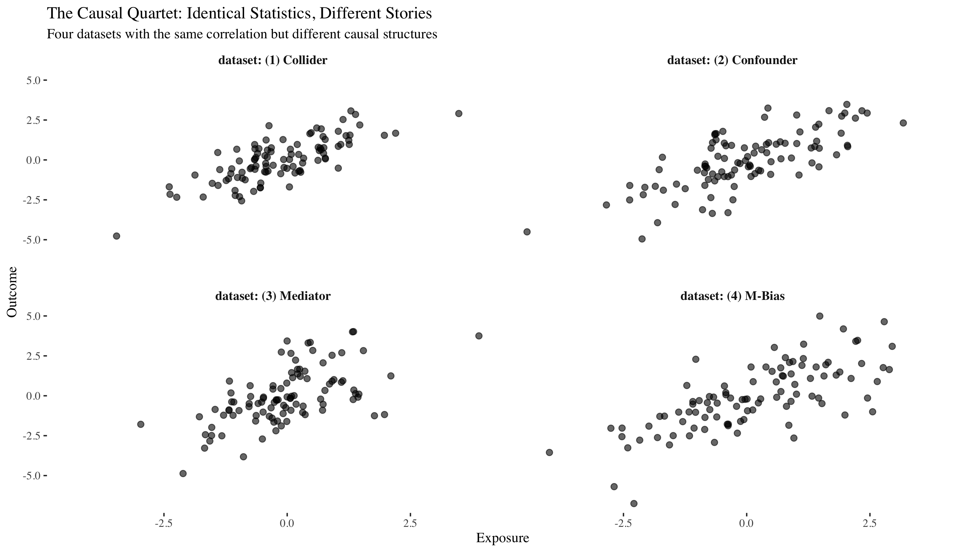
All four datasets have nearly identical means, standard deviations, and correlations. If we only looked at these summary statistics, we might think they're the same data. They look similar, but the underlying causal mechanisms are completely different. To see why, we need to understand Pearl's ladder.
The ladder
Judea Pearl posits that causal reasoning exists on three distinct levels. Each rung requires more sstructure than the one below it, and each rung enables us to answer questions that are impossible at lower levels.
Rung 1: association - The world of pure observation. We ask "what is?" We observe patterns and correlations. This is the domain of traditional statistics. We can compute things like P(Y|X), the probability of Y given that we observe X. Remarkably, even at this rung of the ladder, causal assumptions made explicit can - sometimes - be falsified because different causal relationships result in different implications for conditional distributions between variables.
Rung 2: intervention - The world of action and experiments. We ask "what if I do?" We imagine actively manipulating one variable and seeing what happens to another. This is the domain of randomized controlled trials and policy evaluation. We compute things like P(Y|do(X)), the probability of Y if we force X to take a particular value - in other words, severe X from this causes and set it to a value we choose. In practice, this is often hard to do so the ability to reason about interventions without making them (by modifying the DAG and working out the implications) is very useful.
Rung 3: counterfactuals - The world of imagination and retrospection. We ask "what would have been?" We look at what actually happened and imagine how it would have been different under alternative circumstances. This is the domain of individual-level causal attribution, regret, and responsibility. We compute things like "what would Y have been for this specific individual if X had been different?". Apart from the data and the DAG, we also need to add structural equations (functional relationships) that define how each arrow of the DAG is actualized. Then, we infer something about these functions based on the real data - treatment A failed for Patient 2 tells us something - and thus we can attempt to answer a question like "Would Patient 2 have recovered with treatment B?".
Each rung requires adding something to what we had before. Let's climb the ladder step by step, using the causal quartet as our guide.
Rung 1: association
At the first rung, we're observing the world and looking for patterns. We have data, and we can compute conditional probabilities, correlations, and statistical associations. But we cannot distinguish between causation and correlation. All we can say is "when I see X, I tend to see Y."
What we add: DAG structure
To work at this level, we add a directed acyclic graph (DAG) that represents possible conditional independence relationships. The DAG is just a hypothesis about the structure of dependencies between variables. At this level, the edges don't necessarily mean "causes" - they just mean "statistically dependent."
The four datasets in the causal quartet actually correspond to four simple DAG structures. Let's take a look.
# Dataset 1: Collider (X causes Y, Both cause Z)
dag1 <- dagitty('dag {
exposure -> outcome
exposure -> covariate
outcome -> covariate
}')
# Dataset 2: Common cause / Confounder (Z causes both X and Y)
dag2 <- dagitty('dag {
covariate -> exposure
covariate -> outcome
exposure -> outcome
}')
# Dataset 3: Mediation / Chain (X causes Z, Z causes Y)
dag3 <- dagitty('dag {
exposure -> covariate -> outcome
}')
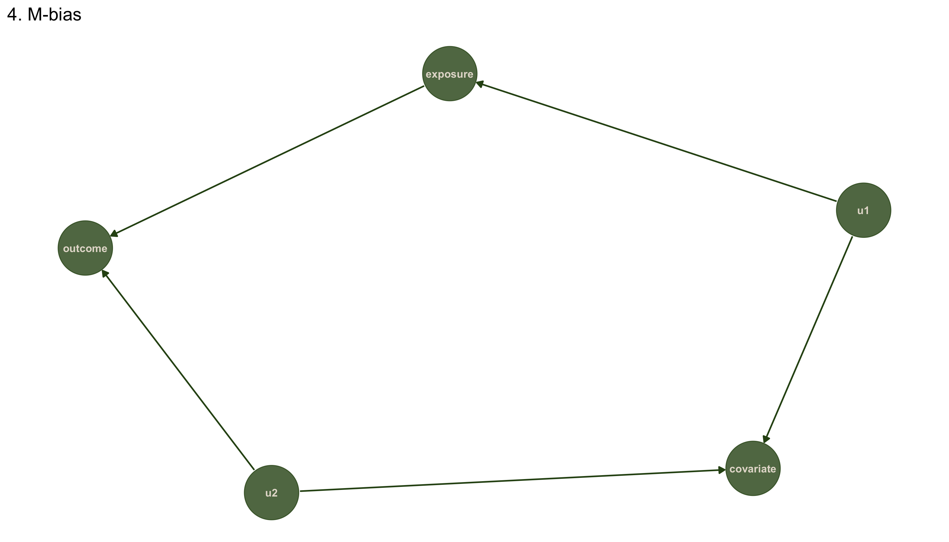
# Dataset 4: M-bias (X and Y both cause Z)
dag4 <- dagitty('dag {
u1 -> covariate
u1 -> exposure -> outcome
u2 -> covariate
u2 -> outcome
}')
p1 + p2 + p3 + p4 +
  plot_layout(ncol = 2, nrow = 2)
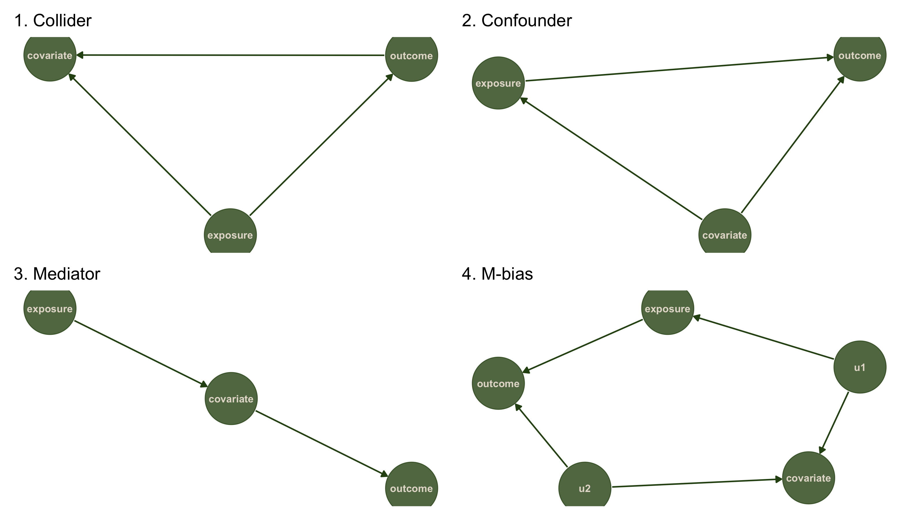
While the headline stats are the same, the 4 data sets represent very different causal structures, seen above.
Testing DAGs against data
In a typical situation, the DAG is an explicit set of assumptions about the world generated by the scientist, and these need to be tested against the data. The key insight of the first rung of causation is that different DAG structures imply different patterns of conditional independence. Even though x and y are correlated in all four datasets, they have different relationships when we condition on the third variable z.
We can use the d-separation criterion (two variables are independent given your controls if no path between them can transmit information) to derive testable implications. The dagitty package does this automatically for us with the impliedConditionalIndependencies function.
## DAG 1 (Collider) implies:
## DAG 2 (Confounder) implies:
## DAG 3 (Mediation) implies:
## exps _||_ otcm | cvrt
## DAG 4 (M-bias) implies:
## cvrt _||_ exps | u1
## cvrt _||_ otcm | exps, u2
## cvrt _||_ otcm | u1, u2
## exps _||_ u2
## otcm _||_ u1 | exps
## u1 _||_ u2
We see that DAGs 1,2 can't be falsified at Rung 1, since there are no conditional implications we can test (and which could potentially be false).
Before we start testing our DAG hypotheses with data, we need to understand what we're actually testing and how to interpret the results. This is subtle because the logic is inverted from typical hypothesis testing. The testing procedure works as follows:
- Extract all conditional independence implications from the DAG using d-separation
- For each implication of the form \(X \perp Y \mid Z\) (for example):
- Regress \(X\) on \(Z\) to get residuals \(r_X\)
- Regress \(Y\) on \(Z\) to get residuals \(r_Y\)
- Test whether \(\text{cor}(r_X, r_Y) = 0\)
- Return a p-value for each test
Interpreting the results:
The null hypothesis \(H_{\phi}\) is that the variables ARE conditionally independent (as the DAG claims). Therefore:
- High p-value (> 0.05): We fail to reject \(H_{\phi}\). The conditional independence holds in the data. The DAG's prediction is not contradicted. The test passes!
- Low p-value (< 0.05): We reject \(H_{\phi}\). The conditional independence is violated. The DAG's prediction is contradicted. The test fails.
Passing all tests does not prove the DAG is correct. Multiple different DAG structures can imply the same set of conditional independencies (these are called "Markov equivalent" DAGs). What we can do is falsify DAG structures that make predictions contradicted by the data. On rung 1, we can use conditional independence testing to rule out impossible causal structures, but we cannot definitively prove which structure is correct from observational data alone.
## [1] "The implications: "
## cvrt _||_ otcm | exps
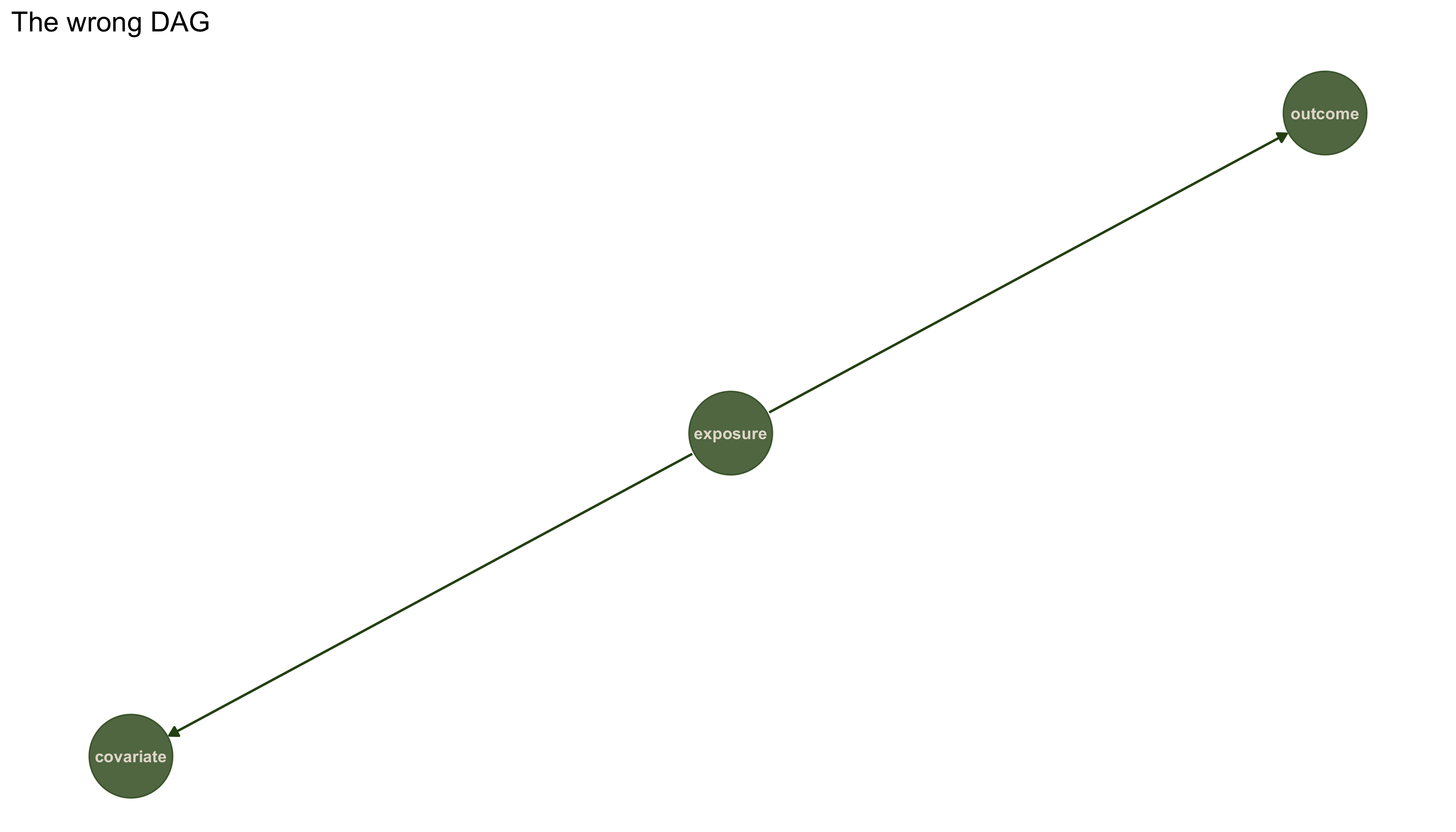
Testing fork structure against dataset 3 (wrong structure):
results3_wrong <- localTests(dag3_wrong, data3, type = "cis")
## Warning in cov2cor(cov(data)): diag(V) had non-positive or NA entries; the
## non-finite result may be dubious
print(results3_wrong)
##                        estimate      p.value      2.5%     97.5%
## cvrt _||_ otcm | exps 0.7605758 1.452368e-22 0.6732402 0.8750805
The test fails! Dataset 3 is not consistent with a fork structure. Instead, it follows a chain structure where x causes z and z causes y. Let's verify that the correct structure fits. Testing chain structure (x -> z -> y) against dataset 3:
results3 <- localTests(dag3, data3, type = "cis")
## Warning in cov2cor(cov(data)): diag(V) had non-positive or NA entries; the
## non-finite result may be dubious
print(results3)
##                          estimate p.value      2.5%     97.5%
## exps _||_ otcm | cvrt 0.002031441 0.98412 -0.195478 0.1993846
The chain structure fits dataset 3...
Limitations of rung 1
"Correlation is not causation" is only the the beginnign of the story. We can use conditional independence testing to falsify causal structures that are inconsistent with the data.
But we cannot prove that any particular structure is correct, we can only show that some structures are inconsistent with the data. Moreover, we cannot distinguish between correlation and causation just from observational data. The edges in our DAGs could represent predictive relationships rather than causal ones.
To go further, we need to climb to the second rung.
Rung 2: intervention
At the second rung, we move from passive observation to active manipulation. We imagine or actually perform interventions where we force a variable to take a particular value and observe what happens to other variables. This is the world of experiments, policies, and "what if I do?" questions. In pragmatic terms, we estimate the actual causal effect of changing a treatment on the outcome.
What we add: causal interpretation
The key addition at rung 2 is semantic: we now interpret the edges in our DAG as representing direct causal relationships, not just statistical dependencies. When we write \(x \rightarrow y\), we mean "x directly causes y," not just "x predicts y."
We add a new mathematical operator: do(X = x), which represents forcing X to take the value x. This is different from observing X = x. When we intervene, we perform graph surgery by removing all incoming edges to X, reflecting the fact that we've overridden X's normal causes.
Estimating direct and total causal effects
Here we estimate causal effects by asking: "What would happen to the outcome if we intervened to set exposure to a specific value?"
In Pearl's do-calculus notation, we write this as \(\mathbb{E}[Y \mid do(X = x)]\) - the expected value of \(Y\) when we set \(X\) to \(x\) (rather than just observe \(X = x\)). We target \(\mathbb{E}[Y \mid do(X = x)]\). The total effect (ATE) is
A direct effect can be defined as a controlled direct effect
or as a natural direct effect (which requires stronger assumptions).
So, given a DAG, which variables should one control for to estimate \(\mathbb{E}[Y \mid do(X)]\) from observational data? This is where the adjustment formula comes in, under certain conditions (backdoor criterion satisfied - set of variables blocks all backdoor paths from exposure to outcome and contains no descendants of exposure),
In practice with regression, if we adjust for the right \(Z\), the coefficient on \(X\) estimates the causal effect (ATE).
The daggity package has several helpful functions:
- The
pathsfunction lists all paths from exposure to outcome and tells us if they are open or not:
p4
paths(dag4, "exposure", "outcome")
## $paths
## [1] "exposure -> outcome"
## [2] "exposure <- u1 -> covariate <- u2 -> outcome"
##
## $open
## [1]  TRUE FALSE
- The
adjustmentSetsfunction tells us what to control for when estimating direct and total effets:
adjustmentSets(dag4, exposure = "exposure", outcome = "outcome",
                             effect = "direct", type = "minimal")
## {}
adjustmentSets(dag4, exposure = "exposure", outcome = "outcome",
                             effect = "total", type = "minimal")
## {}
which tells us that we don't need to control for anything in DAG-4 to estimate the total and direct effects. Moreover, since the only backdoor path is closed, the total and direct effects are going to be the same for this DAG.
data4 <- causal_quartet |>
  filter(dataset == "(4) M-Bias") |>
  select(exposure, outcome, covariate, u1, u2)
lm(outcome ~ exposure, data4)
##
## Call:
## lm(formula = outcome ~ exposure, data = data4)
##
## Coefficients:
## (Intercept)     exposure
##     -0.2175       1.0041
Lets see this for the mediator (DAG-3) (where we know the direct effect should be 0, since there is no arrow going from exposure to outcome):
p3
adjustmentSets(dag3, exposure = "exposure", outcome = "outcome",
                             effect = "direct", type = "minimal")
## { covariate }
adjustmentSets(dag3, exposure = "exposure", outcome = "outcome",
                             effect = "total", type = "minimal")
## {}
So, to estimate the direct effect we need to condition on the covariate:
lm(outcome ~ covariate + exposure, data3)
##
## Call:
## lm(formula = outcome ~ covariate + exposure, data = data3)
##
## Coefficients:
## (Intercept)    covariate     exposure
##    0.014874     1.067466     0.002474
and we see that the direct effect of exposure on outcome is ~0. For the total effect, we don't need to control for anything:
lm(outcome ~ exposure, data3)
##
## Call:
## lm(formula = outcome ~ exposure, data = data3)
##
## Coefficients:
## (Intercept)     exposure
##   -0.007654     0.995610
So much linear regression!
While we have used lm() throughout, the DAG-based adjustment strategy (what to control for) remains valid regardless of the statistical method. The DAG tells you what to adjust for, the statistical method determines how to adjust for it.
When relationships between variables arenon-linear, methods like splines or generalized additive models (GAMs) via the mgcv package can be used. These allow smooth, flexible relationships while remaining interpretable - one can visualize exactly how covariates affect the outcome. For example:
gam(outcome ~ exposure + s(covariate), data = data) estimates the causal effect of the exposure while relaxing the.
Beyond controlling directly in a regression, there are other techniques like propensity score methods
(matching or weighting by the probability of treatment) via packages like MatchIt or WeightIt. For a "best of both worlds" approach, doubly robust methods combine outcome modeling with propensity scores—you get the correct answer if either model is right (see AIPW package). This relies on balancing the groups (treated/untreated) on covariates by matching similar entities or reweighting the sample, so comparing outcomes is like comparing a randomized trial.
When treatment effects vary across individuals, causal forests from the grf package use machine learning to estimate personalized treatment effects non-parametrically. See Athey & Wager (2019) for the methodology, or the excellent documentation that comes with the grf package
All these methods relax parametric assumptions (linearity, functional form) but cannot escape the fundamental causal assumptions—namely, that your DAG is correct and all confounders are measured. As Judea Pearl emphasizes: "no causes in, no causes out"—no statistical technique can create causal knowledge from purely observational data if the DAG is wrong. The fanciest machine learning model with the wrong adjustment set will give worse answers than simple linear regression with the right one.
The power and limits of rung 2
At rung 2, we can answer policy questions and predict the effects of interventions. We can distinguish between genuine causal effects and spurious correlations due to confounding. This is very useful for science and decision-making.
We can tell the average effect of intervening on x in the population: \(P(Y|do(X))\) tells us what would happen on average if we forced X for everyone. But we cannot tell you what would have happened for a specific individual who actually experienced one value of X. We cannot answer "what if things had been different for this person?"
To answer that question, we need to climb to the third rung.
Rung 3: counterfactuals
At the third rung, we move from population-level predictions to individual-level explanations. We look at what actually happened to a specific person or instance and ask "what would have been different if...?" This is the domain of regret, responsibility, attribution, and retrospection.
What we add: functional mechanisms
The key addition at rung 3 is the specification of functional equations that describe how each variable is generated from its causes. We move from a DAG (which just shows which variables affect which) to a Structural Causal Model (SCM), which specifies the mechanisms.
For each variable, we write:
where \(f_i\) is a function and \(U_i\) represents all the unmeasured factors (noise, randomness, individual variation) that affect \(X_i\).
This is a big step up in specificity. At rung 2, we only needed to know the graph structure. At rung 3, we need to know the actual functional form of how causes produce effects.
What we can do: individual counterfactuals
Let's work with dataset 3 (the chain structure) since it has a clear causal mechanism we can estimate. The data was actually generated from a specific structural model. Let's estimate that model and use it to answer counterfactual questions.
## Structural equations:
## covariate = -0.021 + 0.93*exposure + u_covariate
## outcome = 0.015 + 1.069*covariate + u_outcome
Now suppose we observe a specific individual with exposure = 1.5, covariate = 2.0, outcome = 3.5. We want to answer: "What would outcome have been for this individual if exposure had been 2.5 instead?"
This is a counterfactual question. To answer it, we use Pearl's three-step procedure:
- Abduction: Given what we observed, infer the values of the unobserved noise terms \(U_{covariate}\) and \(U_{outcome}\) for this specific individual
- Action: Modify the structural equations to reflect the intervention (set exposure = 2.5)
- Prediction: Compute what outcome would have been using the modified equations and the inferred noise terms
# Observed values for one individual
observed_exposure <- 1.5
observed_covariate <- 2.0
observed_outcome <- 3.5

# Step 1: Abduction - infer the noise terms
u_covariate <- observed_covariate - predict(model_x_to_z, newdata = tibble(exposure = observed_exposure))
u_outcome <- observed_outcome - predict(model_z_to_y, newdata = tibble(covariate = observed_covariate))

# Step 2: Action - set x to counterfactual value
counterfactual_exposure <- 2.5

# Step 3: Prediction - compute counterfactual y
# First, compute what z would have been
counterfactual_covariate <- predict(model_x_to_z,
                            newdata = tibble(exposure = counterfactual_exposure)) + u_covariate

# Then, compute what y would have been
counterfactual_outcome <- predict(model_z_to_y,
                           newdata = tibble(covariate = counterfactual_covariate)) + u_outcome
## Summary:
## Observed: x = 1.5 , y = 3.5
## Counterfactual: if x had been 2.5 , y would have been 4.494
## Effect for this individual: 0.994
The Connection to Bayesian Inference
What we did in step 1 (abduction) looks a lot like Bayesian inference. We observed some data and used it to infer the values of unobserved variables (the noise terms). In a Bayesian framework, we would treat the noise terms as latent variables and compute their posterior distribution given the observed data. Then, to compute counterfactuals, we would sample from this posterior and simulate what would have happened under different interventions.
This is exactly the approach taken in Richard McElreath's "Statistical Rethinking", where he shows how to use Bayesian inference to compute counterfactuals in structural causal models. The generative model (the SCM) becomes the inference target, and counterfactual reasoning becomes a form of posterior prediction under modified models.
The Power and Limits of Rung 3
At rung 3, we can answer questions about individual instances and attribute causation at the finest grain. We can reason about responsibility, regret, and explanation. We can say not just "smoking causes cancer on average" but "Bob's cancer was caused by his smoking."
But this power comes at a price. We need much more information than at lower rungs. Specifically, we need:
- The correct causal graph (rung 2 requirement)
- The functional form of how causes produce effects
- The distribution of unobserved factors
These requirements are often difficult or impossible to satisfy with observational data alone. We typically need strong assumptions about functional forms (linearity, additivity, etc.) or additional data from experiments.
Returning to the Rudder Paradox
Let's generate some data that mimics the rudder situation and see how each rung of the ladder handles it.
# Simulate the rudder situation
set.seed(123)
n <- 500

# Generate data
# W = wind (unobserved!)
# R = rudder position (sailor adjusts to counteract wind)
# D = direction (affected by both wind and rudder)

W <- rnorm(n, mean = 0, sd = 1)  # Wind is unobserved
R <- -1 * W + rnorm(n, 0, 0.1)  # Rudder counteracts wind
D <- 0.5 * W + 0.5 * R + rnorm(n, 0, 0.1)  # Direction depends on both

rudder_data <- tibble(
  W = W,  # We'll pretend we don't observe this
  R = R,
  D = D
)

# The true causal structure
rudder_dag <- dagitty('dag {
  W -> R
  W -> D
  R -> D
}')

rudder_dag |>
  tidy_dagitty() |>
  ggplot(aes(x = x, y = y, xend = xend, yend = yend)) +
  geom_dag_point(color = "#2D5016", size = 20, alpha = 0.8) +
  geom_dag_text(color = "#E5DDD1", size = 3.0) + geom_dag_edges(edge_colour = "#2D5016") +
  ggtitle(paste("Rudder problem adjustment set ", adjustmentSets(rudder_dag, exposure = "R", outcome = "D", effect = "total", type = "minimal"))) +
  theme_dag()
Associational analysis
Since we only have observational data on R and D (we can't see the wind W). Let's look at their correlation.
## Correlation between rudder (R) and direction (D): 0.022
## `geom_smooth()` using formula = 'y ~ x'
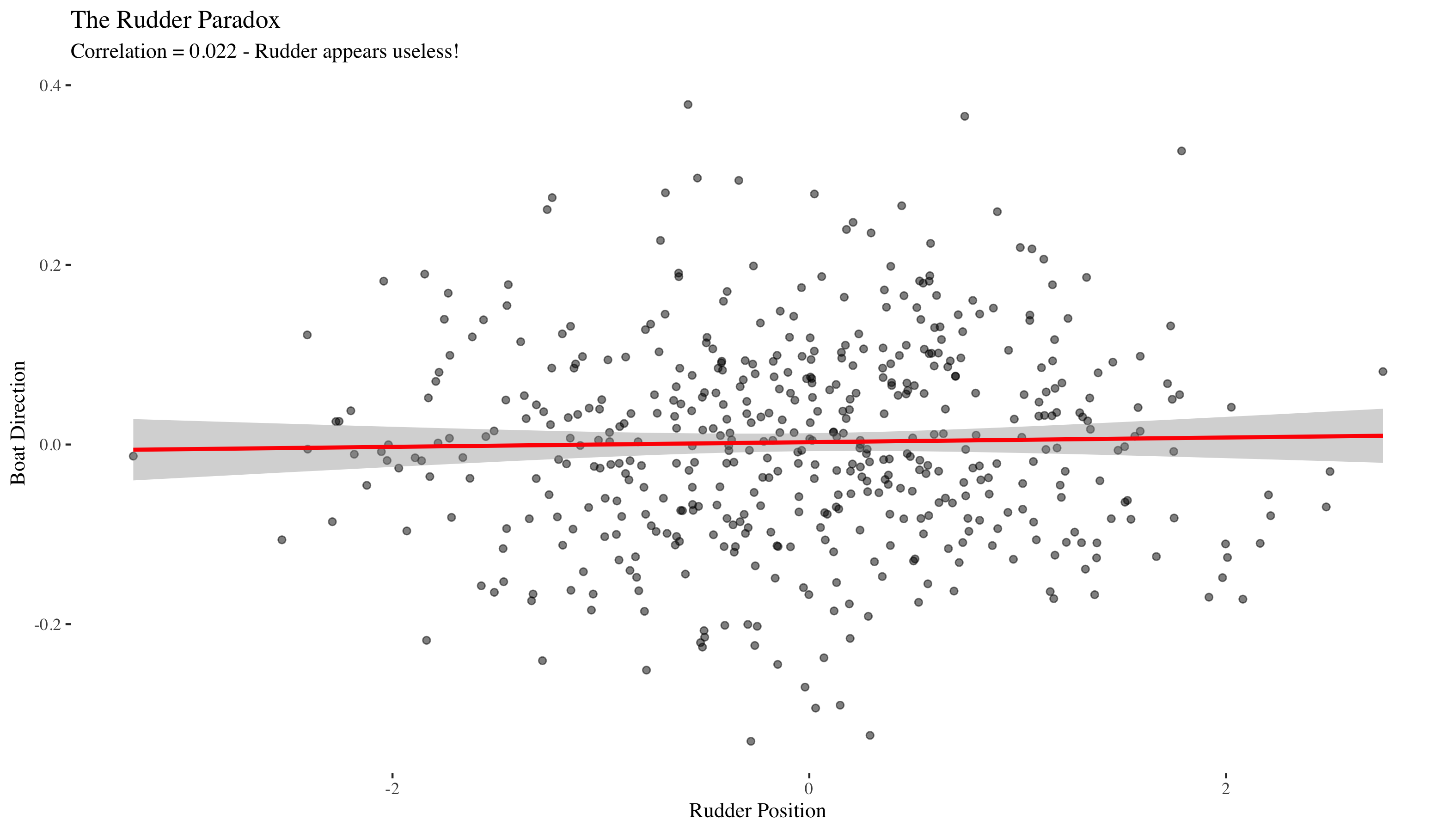
The correlation is near zero! We would conclude (incorrectly) that the rudder doesn't affect the boat's direction. The problem is confounding by the unobserved wind W. The wind affects both R and D in opposite ways, misleading us when we don't account for it.
adjustmentSets(rudder_dag, exposure = "R", outcome = "D",
                             effect = "direct", type = "minimal")
## { W }
To answer this correctly using the adjustment formula, we would need to condition on W (the wind). When W is unobserved, we can't apply the standard backdoor adjustment. However, if we did have access to wind direction W, we could correctly estimate the causal effect - the DAG tells us what we need to measure (wind) to estimate the causal effect of rudder on direction.
# If we could observe W, we could adjust for it
model_adjusted <- lm(D ~ R + W, data = rudder_data)
# Compare to the naive (wrong) estimate
model_naive <- lm(D ~ R, data = rudder_data)
## True causal effect of rudder on direction (adjusting for wind):
##         R
## 0.5531443
##
## Naive estimate (not adjusting for wind):
##          R
## 0.00259491
When we properly adjust for the confounding wind, we see that the rudder has a substantial causal effect (around 0.5) on direction. The naive analysis severely underestimates this effect because it doesn't account for the confounding.
In a real experiment, we could reveal this by randomizing the rudder position (removing the endogeneity). If we forced the rudder to different positions (breaking the W → R link), we would see the true causal effect.
Further reading:
- Causal Inference: What If by Hernán & Robins (free online textbook).
- Causal Inference in R another free online textbook.
- Causal Inference: The Mixtape by Cunningham (free, R and Stata code).
causalworkshopR package with tutorials.