 p. bhogale
 This post is code for the demo associated with a talk on causal inference presented at Fifth Elephant Winter 2025. The video of the talk will be available soon, and I'll link to it here.
We walk through a complete causal inference workflow using real marketing data from the AmExpert 2019 Kaggle competition. The dataset contains transaction records, coupon assignments, and customer demographics from a retail store that ran 18 marketing campaigns. Our goal is to estimate the causal effect of receiving specific coupon types on customer spending during campaign periods.
Our analysis follows the methodology of Langen & Huber (2023), who applied causal machine learning to evaluate coupon effectiveness. Their key finding: drugstore coupons have a significant positive effect on sales, while ready-to-eat food coupons show no significant effect. We replicate this finding using a simplified classical approach, demonstrating how DAG-based identification translates directly into a regression specification.
The Causal Structure
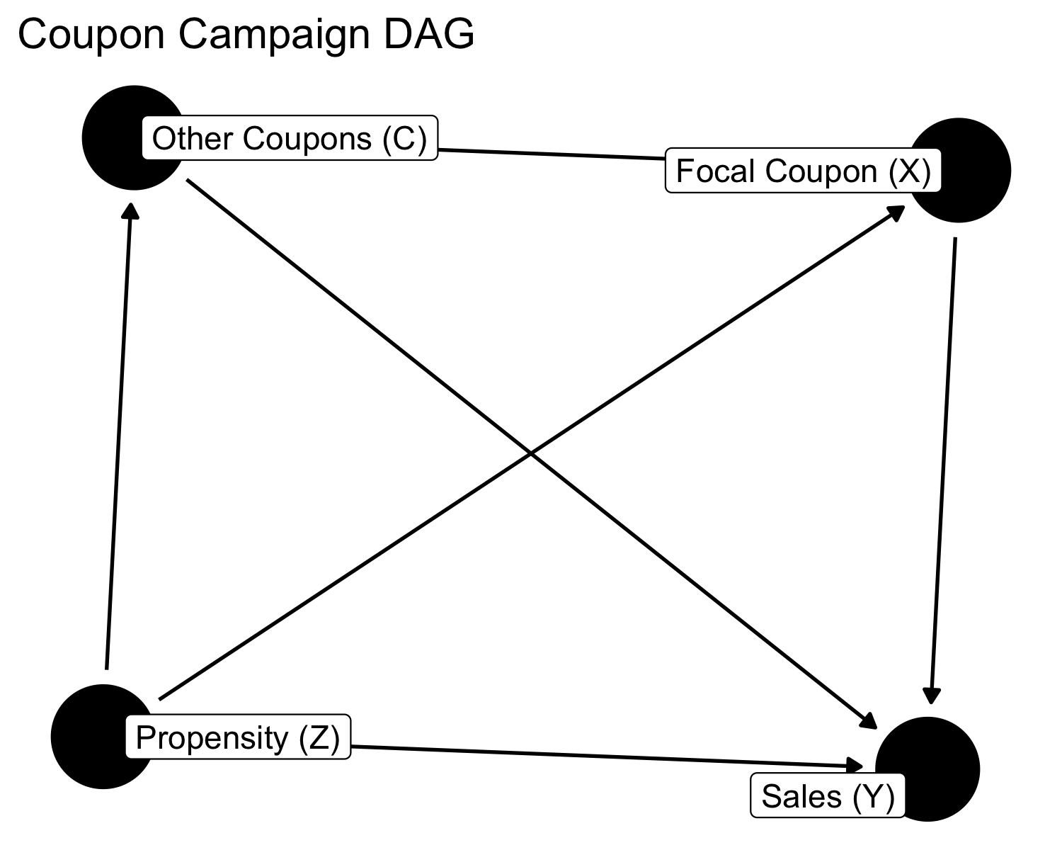
We model the coupon-sales relationship with the following DAG:
# Simple visualization for HTML output
library(ggdag)
dag <- dagify(
  Y ~ X + Z + C,
  X ~ Z + C,
  C ~ Z,
  exposure = "X",
  outcome = "Y",
  labels = c(Y = "Sales (Y)", X = "Focal Coupon (X)",
             Z = "Propensity (Z)", C = "Other Coupons (C)")
)
ggdag(dag, text = FALSE, use_labels = "label") +
  theme_dag_blank() +
  labs(title = "Coupon Campaign DAG")
center
Variables:
- Z (Propensity): Pre-campaign average daily spending—a scalar index of how likely a customer is to buy. High-Z customers are more likely to receive coupons (retailer targeting) and more likely to spend (baseline behavior).
- X (Focal Coupon): Binary indicator for whether the customer received a coupon of the category we're studying (e.g., drugstore).
- C (Other Coupons): Binary indicator for whether the customer received coupons from other categories in the same campaign.
- Y (Sales): Average daily expenditures during the campaign period.
Data Preparation
The dataset consists of six CSV files: train.csv (coupon assignments), campaign_data.csv (campaign dates), customer_transaction_data.csv (purchase records), item_data.csv (product categories), coupon_item_mapping.csv (coupon-to-product mappings), and customer_demographics.csv. We construct a customer × campaign panel where each row contains the propensity index Z, treatment indicators X and C, and outcome Y.
Following Langen & Huber (2023), we compare each coupon category against customers who received no coupons at all (not "no coupon of this type"). This ensures the control group is uncontaminated by other coupon effects. The transaction data contains extreme outliers (wholesale/B2B accounts with transactions in the millions), which we filter at the 95th percentile to focus on retail customers.
sample_sizes <- tibble::tibble(
  coupon_type = c("Drugstore", "Ready-to-eat"),
  n           = c(nrow(df_drugstore), nrow(df_ready2eat)),
  treated     = c(sum(df_drugstore$X == 1), sum(df_ready2eat$X == 1)),
  control     = c(sum(df_drugstore$X == 0), sum(df_ready2eat$X == 0))
)

sample_sizes |>
  knitr::kable(
    col.names = c("Coupon type", "N", "Treated (X = 1)", "Control (X = 0)"),
    caption   = "Sample sizes by coupon type and treatment status"
  ) |>
  kableExtra::kable_styling(full_width = FALSE)
| Coupon type | N | Treated (X = 1) | Control (X = 0) |
|---|---|---|---|
| Drugstore | 26577 | 3759 | 22818 |
| Ready-to-eat | 24831 | 2013 | 22818 |
Traditional Causal Inference Workflow
DAG Specification and Identification
We have already defined the DAG in dagitty and now, we can use dosearch to verify that the causal effect is identifiable:
# Check adjustment sets
dagitty::adjustmentSets(dag, exposure = "X", outcome = "Y")
## { C, Z }
# Verify with dosearch
data_spec  <- "P(X, Y, Z, C)"
query_spec <- "P(Y | do(X))"

dosearch::dosearch(data_spec, query_spec, dag)
## \sum_{C,Z}\left(p(C,Z)p(Y|X,C,Z)\right)
The backdoor criterion confirms that conditioning on {Z, C} blocks all non-causal paths from X to Y. This translates directly to the regression specification:
where \(\hat{\tau}\) estimates the Average Treatment Effect (ATE) under the assumption of no unmeasured confounding.
ATE Estimation
Drugstore Coupons
# Naive estimate (no adjustment - confounded!)
m_drug_naive <- lm(Y ~ X, data = df_drugstore)
naive_drug <- broom::tidy(m_drug_naive, conf.int = TRUE) |>
  dplyr::filter(term == "X") |>
  dplyr::mutate(model = "Naive")

# Adjusted estimate (backdoor criterion satisfied)
m_drug_adj <- lm(Y ~ X + Z + C_other, data = df_drugstore)
adj_drug <- broom::tidy(m_drug_adj, conf.int = TRUE) |>
  dplyr::filter(term == "X") |>
  dplyr::mutate(model = "Adjusted")

lmtest::coeftest(m_drug_adj, vcov = sandwich::vcovHC(m_drug_adj, type = "HC1"))
##
## t test of coefficients:
##
##                Estimate  Std. Error  t value Pr(>|t|)
## (Intercept)  50.6436723   0.9961180  50.8410  < 2e-16 ***
## X            25.2709931  10.7057762   2.3605  0.01826 *
## Z             0.7276585   0.0053766 135.3369  < 2e-16 ***
## C_other     -26.4019676  10.8264763  -2.4386  0.01475 *
## ---
## Signif. codes:  0 '***' 0.001 '**' 0.01 '*' 0.05 '.' 0.1 ' ' 1
Ready-to-Eat Coupons
# Naive estimate (no adjustment - confounded)
m_ready_naive <- lm(Y ~ X, data = df_ready2eat)
naive_ready <- broom::tidy(m_ready_naive, conf.int = TRUE) |>
  dplyr::filter(term == "X") |>
  dplyr::mutate(model = "Naive")

# Adjusted estimate (backdoor criterion satisfied)
m_ready_adj <- lm(Y ~ X + Z + C_other, data = df_ready2eat)
adj_ready <- broom::tidy(m_ready_adj, conf.int = TRUE) |>
  dplyr::filter(term == "X") |>
  dplyr::mutate(model = "Adjusted")

lmtest::coeftest(m_ready_adj, vcov = sandwich::vcovHC(m_ready_adj, type = "HC1"))
##
## t test of coefficients:
##
##               Estimate Std. Error  t value Pr(>|t|)
## (Intercept) 50.8415118  1.0130037  50.1889   <2e-16 ***
## X           -0.3656755  2.5331899  -0.1444   0.8852
## Z            0.7265872  0.0055676 130.5037   <2e-16 ***
## ---
## Signif. codes:  0 '***' 0.001 '**' 0.01 '*' 0.05 '.' 0.1 ' ' 1
Comparison: Naive vs Adjusted
# Build full comparison table (includes conf.low/conf.high for plot)
comparison_table <- dplyr::bind_rows(
  naive_drug  |> dplyr::mutate(coupon_type = "Drugstore"),
  adj_drug    |> dplyr::mutate(coupon_type = "Drugstore"),
  naive_ready |> dplyr::mutate(coupon_type = "Ready-to-eat"),
  adj_ready   |> dplyr::mutate(coupon_type = "Ready-to-eat")
) |>
  dplyr::select(coupon_type, model, estimate, conf.low, conf.high, p.value)

# Display table with kableExtra (only key columns)
comparison_table |>
  dplyr::select(coupon_type, model, estimate, p.value) |>
  knitr::kable(
    col.names = c("Coupon Type", "Model", "Estimate", "p-value"),
    digits = c(0, 0, 2, 4),
    caption = "Naive vs Adjusted Effect Estimates by Coupon Type"
  ) |>
  kableExtra::kable_styling(full_width = FALSE, bootstrap_options = c("striped", "hover")) |>
  kableExtra::row_spec(c(2, 4), bold = TRUE, color = "steelblue")
| Coupon Type | Model | Estimate | p-value |
|---|---|---|---|
| Drugstore | Naive | 29.94 | 0.0000 |
| Drugstore | Adjusted | 25.27 | 0.0021 |
| Ready-to-eat | Naive | 25.95 | 0.0000 |
| Ready-to-eat | Adjusted | -0.37 | 0.8788 |
# Plot with error bars (uses conf.low/conf.high from full table)
comparison_table |>
  ggplot(aes(x = coupon_type, y = estimate, color = model, shape = model)) +
  geom_point(size = 3, position = position_dodge(width = 0.4)) +
  geom_errorbar(aes(ymin = conf.low, ymax = conf.high),
                width = 0.2, linewidth = 1., position = position_dodge(width = 0.4)) +
  geom_hline(yintercept = 0, linetype = "dashed", color = "gray50", linewidth = 0.8) +
  scale_color_manual(values = c("Naive" = "firebrick3", "Adjusted" = "steelblue")) +
  labs(
    title = "Naive vs Adjusted Effect Estimates",
    subtitle = "Adjusting for confounders {Z, C} changes effect estimates",
    x = "Coupon Type",
    y = "Effect on Daily Spend",
    color = "Model", shape = "Model"
  ) +
  theme_tufte(base_size = 14) +
  theme(
    legend.position = "bottom",
    plot.title = element_text(size = 20, face = "bold"),
    plot.subtitle = element_text(size = 14),
    axis.title = element_text(size = 16),
    axis.text = element_text(size = 14),
    legend.text = element_text(size = 12),
    legend.title = element_text(size = 14)
  ) -> p
p
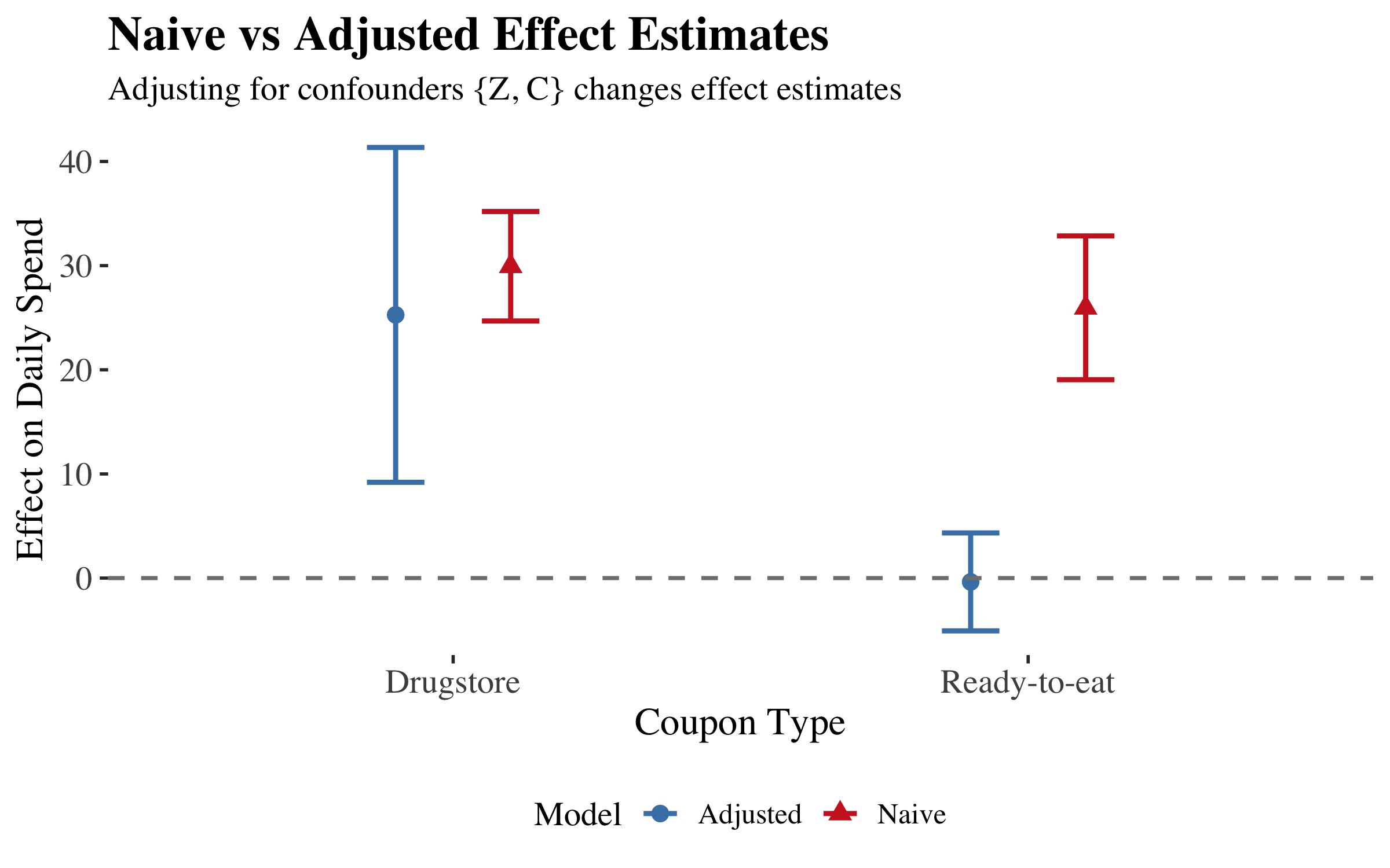
Interpretation: Consistent with Langen & Huber (2023), we find that drugstore coupons have a larger positive effect on sales, while ready-to-eat coupons show no effect.
Causal Machine Learning
The classical regression approach above assumes a linear, additive relationship between covariates and outcome. Langen & Huber (2023) use a causal ML approach to the problem -- Causal forests (Wager & Athey, 2018; Athey, Tibshirani & Wager, 2019) relax this assumption while maintaining the same identification logic.
We will explore this further in the next post.